Download Test Case

Modal analysis of a unit under test yields important information about the natural frequencies, damping coefficients and mode shapes to optimize its design and improve its structural behavior. The modal parameters of a test unit and its mechanical properties will help users understand the vibration characteristics during operating conditions.

The case described in this article examines the modal characteristics of a satellite model acquired from performing experimental modal analysis. A hammer impact test was carried out with two teardrop uni-axial accelerometers (mounted in different directions) to study the modal behavior. The roving excitation method assists in completely avoiding the potential mass loading side effect produced by a roving response procedure. A hard tip was selected to excite the higher frequency modes.

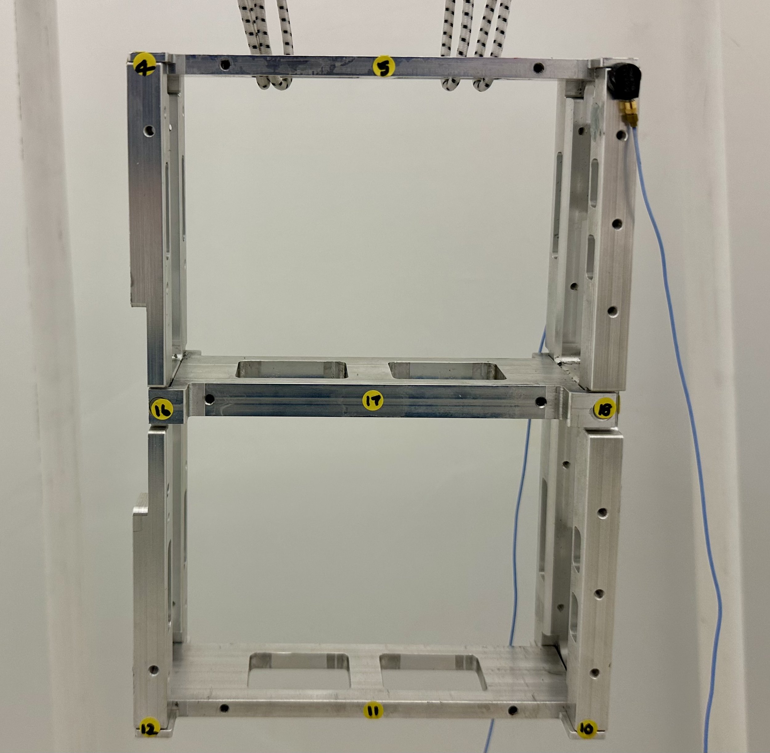
Figure 1. Hammer Impact Modal Test of the Satellite Model

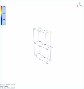
A geometry mesh configuration of 18 measurement points is uniformly distributed throughout the satellite model to achieve good spatial resolution for the mode shapes. Flexible bands and bungee cords were used to suspend the satellite model vertically to imitate a free-free boundary condition (as shown in the experimental setup). The tiny uni-axial teardrop accelerometers were fixed to two locations (in X and Y directions) and the impact hammer was roved through the points to acquire 108 FRFs at the 18 desired measurement locations. The excitation force and response accelerations in the X, Y and Z directions were measured to obtain the 3D mode shapes.

modal measurements — Figure 2. Satellite Model Geometry

A sampling rate of 6.4 kHz was set since this satellite model has modes in a higher frequency range. A block size of 4096 was selected to ensure the response decays naturally and windowing is not required. A fine frequency resolution of 1.5625 Hz is produced with these configuration settings. Measurements of higher accuracy and reduced noise are obtained by linearly averaging 3 blocks of data at each measurement DOF.

The hammer impact excitation imparts energy across a broad frequency range of 2.9 kHz. With this setup, there will be no leakage and a uniform window can be selected.

hammer impact measurement — Figure 3. Hammer Impact Measurement of the Satellite Model

The coherence plot helps validate the measurement results. The preceding screenshot illustrates a good example of the results. The valleys in the coherence plot occur at the anti-resonances which indicates that the response level is relatively lower at these corresponding frequencies. Overall, the inputs and outputs are well correlated within the desirable frequency range.

The FRF measurement displays several dominant peaks in the 0-2900 Hz frequency band. Several modes can be identified when overlapping the 108 measured FRFs. The peaks are well aligned which indicates good measurement results and the lack of a mass loading effect.

modal data selection — Figure 4. Modal Data Selection tab showing the magnitude and phase part of all overlapped FRFs

The Complex Mode Indicator Function (CMIF) was used to locate the modes in the desired frequency range. (2 CMIFs were produced for 2 references.) In addition, the summed FRF was also observed to identify the modes. The Poly-X method was used to curve-fit the FRFs and extract thirteen flexible modes within the desired frequency range.

modal stability diagram — Figure 5. Stability Diagram for the thirteen flexible modes

The Auto-MAC matrix assisted in validating the results. The following Auto-MAC matrix shows that the modes are orthogonal to each other (low off-diagonal elements) and are uniquely identified (high diagonal elements). Mode 10 and 12 have some similarity and increasing the number of measurement points (better spatial resolution) will help users to understand the higher order modes.

The animation of the thirteen mode shapes associated with the stable physical poles is shown below. Since the satellite model is asymmetric (right side of the model has more thickness), some local modes (right side of the model having relatively more stiffness) can also be observed along with the global modes. Modes that animate the torsion and bending deformations of the satellite model in-phase and out-of-phase along the different axes can also be observed.

Modes 1 and 2 shows the torsional deformation (about Z axis) of the satellite model.

Modes 3 and 4 animates the bending motion of the satellite model along the sideway (Y axis) and forward directions (X axis) respectively.

Mode 5 shows local bending of the bottom panel of the satellite model. Mode 6 shows the global bending deformation of the panel along the vertical direction (Z axis).