

The classic Gaussian PDF is plotted below.

To appreciate this point, we repeat the Gaussian PDF plot using a logarithmic vertical axis. This scaling is frequently done in vibration work, but rarely shown in statistic texts.

If an experimental measurement matches the Gaussian PDF model, the Gaussian model can then be used to draw many important inferences about the measurement. Many statistical curve-matching tests are available to establish if a measurement is Gaussian. These include the Kolmogorov-Smirnov (KS), Shapiro-Wilk and Anderson-Darling tests. For practical purposes, most well-fixtured and well-conducted random shake tests will produce data that pass any of these model-matching statistical tests for Gaussian behavior.
Important conclusions that result from deeming a measured Control acceleration “Gaussian” include:

Further, we find that if a time-history is Gaussian, the real and imaginary components of its Fourier Transform are also (independently) Gaussian distributed variables. Further, the vector resultant magnitude of those Gaussian components exhibits a different PDF; the spectral magnitude is Rayleigh distributed. Of far greater interest is that the sum of the squares of the real and imaginary components (the power spectrum magnitude) is a Chi-square (X2)distributed variable, as is the variance.
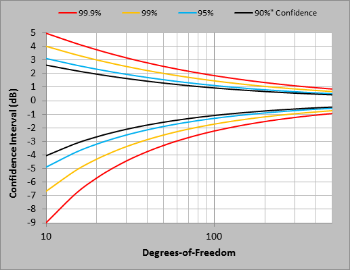
Knowing that the Control PSD has χ2 distributed spectral magnitude allows construction of a confidence interval about any g2/Hz value. The curves above illustrate statistically reasonable bands of variation (±dB) for a g2/Hz spectral value with regard to two variables: Confidence and Degrees-of-Freedom. Statistical Confidence is usually expressed as a percentage. For example, 99.9% Confidence is shorthand for saying 99.9% of the spectral Lines in a PSD will be within the curve-specified upper and lower bounds. So if you average using 200 DOF, you are 90% certain that all of your PSD measured magnitudes are correct within ± 1 dB. We have just begun to scratch the surface of the things that can be learned and ascertained about random signals with Gaussian mean and Chi-square variance. But, that is the stuff of future postings!