
Modal Data Acquisition Using the CoCo-80X/90X
Download PDF | © Copyright Crystal Instruments 2017, All Rights Reserved.Contents: 1. Section One | 2. Section Two
Section 1
Introduction
The Modal Data Acquisition (MDA) function for the CoCo-80X/90 allows the user to conveniently acquire modal data. It provides an interactive user interface for testing, which gives the user flexibility to assign geometric DOFs and signal names to data files even during the middle of testing. Data files can then be transferred to the PC with just a few mouse clicks. After the data files are generated, modal analysis can be performed by EDM Modal software from Crystal Instruments.
This document describes a step-by-step process of CoCo MDA function and the use of EDM Modal software as an example for complete modal analysis.
System Set Up
When using the CoCo-80X to perform modal testing, 2, 4, 8 channel versions will support MDA. Even the 16 channel CoCo-90 will support MDA. In this example, we used following equipment and devices:
- PC with Crystal Instruments EDM Modal software
- CoCo-80X/90X Four Channel Signal Analyzer
- Impact hammer (IEPE impact hammers can be powered by CoCo)
- Two IEPE accelerometers
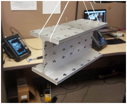
- Test structure: a metal I-Beam
- Suspension bungee cords

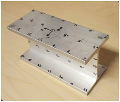

Mark the Degrees of Freedom (DOFs)
First, we create the following meshing DOFs of the I-Beam. In this test, a fixed excitation is selected and the response will be roving through all the measurement DOFs. Meaning that channel 1 will measure the impact force at a fixed location, point 7, +Z direction, channel 2 and channel 3 will rove across all DOFs of the points.
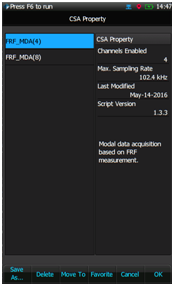
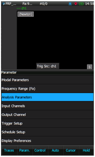
Select Appropriate Configurable Signal Analysis (CSA) Project
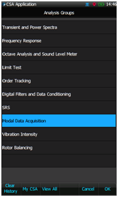
Select the appropriate CSA in the Application group, in this case select FRF_MDA(4). To do so, press Analysis button on the CoCo and enter the Modal Data Acquisition group. See the screenshot below.
Set Up the Parameters
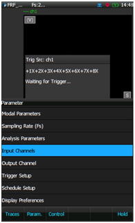
Input Channels
To set up the input channels, select the Input Channels item under Param. Key (F2), then set the appropriate sensitivity for channel 1, channel 2 and channel 3.
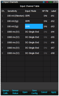
Channel 1 is connected to the impact hammer so therefore the sensitivity should be set to mV/Newton. Channel 2 and 3 are connected to accelerometers with IEPE power enabled.
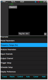
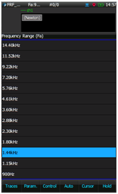
Analysis Frequency Range
This is a very important step and may take a couple of iterations to select the correct analysis frequency range and total capture points. The goal is to select an analysis frequency range that is not too high to show too many modal modes, or too low to miss the important modes. In this test we select the analysis frequency range as 1400Hz.
Analysis Parameters
Select the Analysis Parameters under the Param. (F2) key.
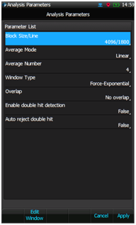
Select the appropriate block size, average mode and average number. Note that the selection of window type must be either Uniform or Force-Exponential for impact hammer testing.
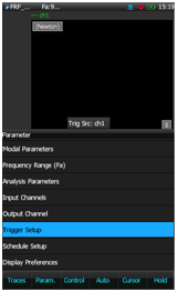
Set-up Trigger
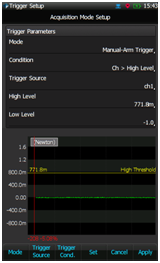
Select the Trigger Setup under Params. (F2) button.
For the impact hammer test, set the following:
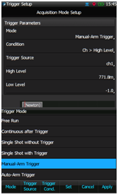
Trigger Mode: Manual Arm Trigger
Trigger Source: channel 1
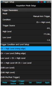
Trigger Condition: Ch1>High Level (rising edge)
Trigger Delay: roughly 5%
Trigger Level: adjust to roughly half the peak value of Ch1

Set Up Modal Parameters
When initially entering the MDA interface, select Modal Parameters under the Param. button (F2).

First, enable block signals to be saved into files. Typically, modal analysis software will only need FRF signals (Frequency Response). However, other signals might also be useful. For example, coherence signals are often used for evaluating the quality of the FRF measurement.
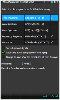
The File Name [xxx] are the file prefix. It can be assigned by the user.
If Auto-save at the completion of averaging is selected, the signals will be automatically saved when each measurement is finished. If this box is not checked, the user must manually save the data files.
If Prompt to save after the completion of each average is checked, there will be a dialog box which prompts the user to confirm the save.
If Saving to SD card is checked, data files will be saved to the SD memory card. Otherwise it will be saved to the internal flash memory. Data can always be transferred from the internal flash memory to the SD memory card at a later time.
Press Next (F5) button to go to the next page.
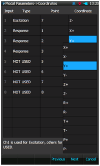
The above screenshot shows the mapping between input channels and the geometric coordinates. Two coordinate types are available: XYZ or RTP. Both coordinate types can be assigned positive or negative directions.
Press Next (F5) button go to the next page.
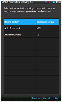
The above page allows the user to set the roving pattern. In theory, the user can set the geometric coordinates manually without automatic roving. But for most tests with hundreds of geometric points, manually entering the coordinates would be too time-consuming. The CoCo MDA provides methods to automate this process.
An advantage of the CoCo MDA is that the automation process can be suspended by the user at any time during testing. This is a necessity because the roving sequence may not be completely regular.
Set the roving pattern to either excitation or response roving.
Set the Increment points. In this example, it is set to 2. Meaning that channel 2 and 3 will measure in a pattern shown below.
Measurement 1: Channel 2= Point 1, Channel 3= Point 2
Measurement 2: Channel 2= Point 3, Channel 3= Point 4
Measurement 3: Channel 2= Point 5, Channel 3= Point 6
…
Section 2
Execute the MDA Test
Now that all the parameters are set, the actual modal test can begin. If the CoCo is in the HOLD mode, press F6 to run. A trigger source window will appear waiting for trigger.
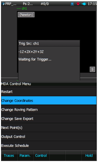
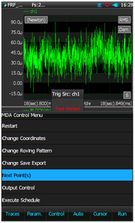
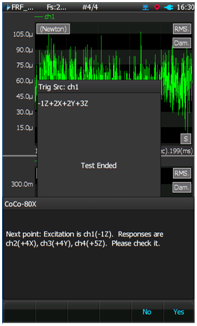
Below are four screenshots showing the control commands for this process:
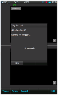
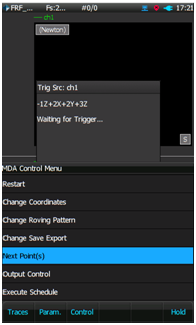

Using the impact hammer, hit point 7 with an appropriate amount of force. Observe the signal qualities. You can carefully examine the signal quality by selecting each trace.
Use the Accept/Reject function to continuously average the signals until the average number is reached.
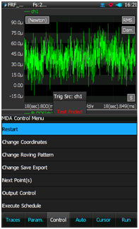
If auto save is set, the signals will be automatically saved to a file with the coordinate information. Otherwise, you must manually press the Save button to save the signals.


Notice in the above picture on the lower left, the small window showing 5 Seconds to save data…
During this five second period, the user has the choice to stop saving the data.
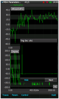
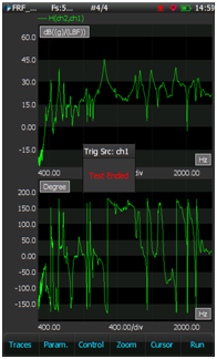
The magnitude and phase signals can be viewed as below.
Under the Control key (F3), you can restart the measurement or manually change the coordinates. If you want to move to the next measurement point, select Next Points.
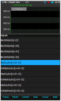
View Files on CoCo
During testing or once finished, you can always view saved data files. Press the File button on the CoCo to view saved files and signals.

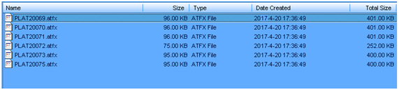
Download Files to PC
After all the measurements are taken, connect the CoCo to a PC with EDM installed. Download the data files to the PC. These data files will be in the ASAM-ODS standard format.
Modal Analysis
EDM Modal is complete modal analysis tool used for modal testing and analysis. For this testing sample, it is used for the parameter identification process of modal analysis.
The software design is based on the process. The main tabs are arranged intuitively based on the operation sequence, from left to right.
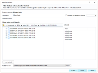
New Test with Data Files Selected
Create a new “Import FRF Data” test using EDM Modal. Select the modal data by browsing to the .atfx files (paired with .dat files), saved to the PC in the previous step.
Build the Geometry
For any structure under test, the geometry editor of the EDM Modal software can be used to construct a geometry model for animation of the mode shapes identified.
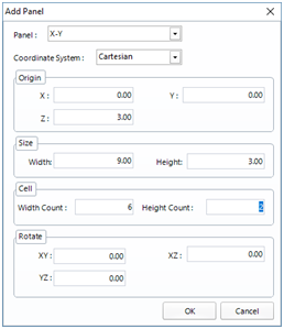
For the I-Beam under test, 3 simple plates can be built first using the panel component. As shown in following, the top plate is on X-Y plane, with the origin at 3 inches along +Z direction. The size and cell define the dimension and number of sections of this plate.
Then, the in-between lines and surfaces from the top as well as bottom plate to the middle plate can be added manually, using the editing tools of the geometry editor.
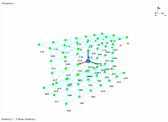
Final geometry is shown as following, with the quad view arrangement.
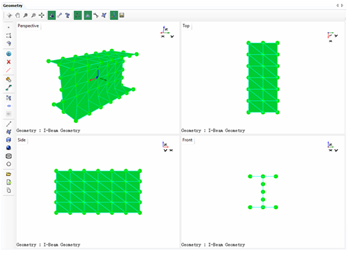
On the top and bottom plate, the measurement is carried out along the Z direction. While on the middle plate, the measurement is carried out along the +Y direction. There are total of 63 points on this I-Beam geometry model.
Modal Data Selection
With the browsed in measurement data (.atfx files) window open, right-click inside the “Data Files” panel, and then select “Open to Modal Data Selection”. The FRF signals of the browsed in data files will be read in and added into the “Modal Data Selection” panel.

The FRF signals from each measurement can be displayed one by one, or all together. The current corresponding response point will be highlighted on the geometry model as a red dot.
Clicking the “Modal Parameters” button, will bring the analysis into next stage: Band Selection.
Band Selection
The band selection has a choice of different types of MIF functions and the FRF Sum. They are used to indicate where the modes, or in other words, natural frequencies are.
The main purpose of the band selection tab is to set the frequency band for the modal parameter identification. The start and end frequency of the analysis band can be set using the band window, or entered directly into the text boxes.

With the band selected and the max order of modes defined, “calculate stabilization” can be clicked to start the curve fitting of the poles. This will bring the software into the next tab, “Stability Diagram”.
Stability Diagram
On the stability diagram, the number of poles are drawn with the mode order increasing from 1 to the max order. The stable poles are illustrated with the green + sign. The stable pole along with a fixed frequency can be selected and used for the next mode shape data fitting.
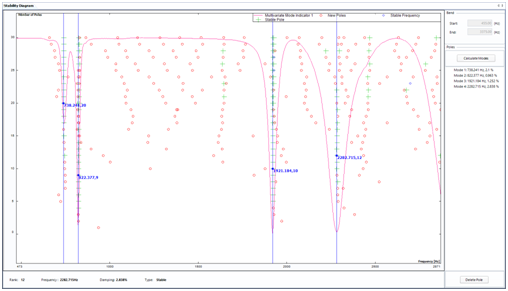
With all the stable poles selected, clicking “Calculate Mode” will bring up the “Mode Shape Save Option” window, as following,
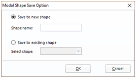
The coming mode shape can be saved to a new shape data file, or saved to an existing shape data file. In general the modal analysis process is done through multiple bands, and the mode data can be saved to an existing shape data file. This will result in one shape data file containing all the mode data over the complete frequency range.
Animation
With the mode saved in the previous stage, EDM Modal software moves onto this Animation tab. The top left panel illustrates the MAC matrix data of the current shape file. The natural frequency and damping of each mode is listed under it. Once a mode is selected for animation, the mode shape data of this mode is listed in the lower left panel.
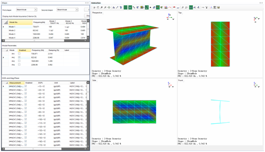
The mode shape animation can be set to different speed and amplitude using the animation control icons. In addition, the different geometry display features can be used to provide a good visual effect of the animation.