
Acoustic Analysis
Crystal Instruments provides a comprehensive range of acoustic measurement systems. Distinct advantages include high channel counts, maximum sampling rates, portability, and patented technology.
Click to view a topic below:
Data Acquisition Systems for Acoustic Measurements and Analysis
Factors to consider when purchasing a DAQ for acoustic measurements:
- Number of channels: The number of required channels will depend on the complexity of the application and the number of sources to be simultaneously measured.
- Maximum sampling rate: The sampling rate must be sufficient to accurately capture the highest frequencies of interest.
- Dynamic range: The dynamic range refers to the range of amplitudes that can be accurately measured by the DAQ system. A wide dynamic range is important to ensure that both weak and strong signals can be accurately measured.
- Compatibility with software: The DAQ system should be compatible with software that allows for easy data visualization, analysis, and manipulation.
- Portability: If the DAQ system will be used in multiple locations or in the field, portability is an important consideration.
While all of Crystal Instruments' data acquisition systems are capable of performing acoustic measurements, certain models may better suit specific application requirements than others.

The GRS was specifically designed for the acquisition of supersonic sound measurements and for remote or autonomous operation.

Spider-80X systems can have 4 to 512 channels. Spider-80Xi systems can have up to 1024 channels.

The CoCo series are handheld DAQs and are ideal for portable applications that require acoustic measurement with 2 to 16 channels.

Spider-20 portable acoustic measurement devices
All systems feature onboard IEPE (ICP®) transducer power capability which allows for direct connection to pre-polarized microphones when used with an ICP microphone pre-amplifier. Traditional condenser microphones are also easily accommodated by connecting the direct voltage signal from the microphone power supply into an input channel. White and pink noise signals can be produced using the waveform generator. This feature is very useful when performing absorption measurements using a speaker.
There are several common post-processing analyses that can be performed on time streams acquired from a data acquisition system for acoustic analysis. Some of these include:
Spectral analysis: This involves using Fourier transforms to convert time domain signals into frequency domain signals, allowing users to visualize the frequency content of the acoustic signal.
Filtering: Filtering can be used to remove unwanted noise or to isolate specific frequency ranges of interest.
Octave analysis: This involves dividing the frequency range into octave bands, which can be useful for assessing noise levels and compliance with noise regulations.
Sound level measurement: Sound level measurements can be used to quantify the overall loudness of a sound or to compare different sound sources.
Statistical analysis: Statistical analysis can be used to assess the variability of acoustic signals or to identify anomalies in the data.

Performing these post-processing analyses allows users to gain a better understanding of the acoustic signals being measured, which can be useful for identifying sources of noise, assessing compliance with regulations, or optimizing the performance of acoustic systems.

Octave Filters
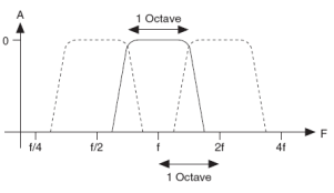
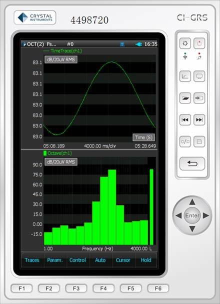
The Fractional Octave Filter Analysis applies a bank of real-time octave filters to the input time streams and generates two types of signals at the same time: fractional frequency band signals, i.e., octave spectra, and the RMS time history of each filter band. The output of each real-time filter bank is in fact a 3D waterfall signal that is arranged in the x-axis as logarithmic frequency and z-axis as time. In the frequency direction, frequency weighting is applied. In the time axis, the time-weighting is applied.
Acoustics Analysis provides 1/N octave analysis using true real-time digital filters that conform to ANSI std. S1.11:2004, Order 3 Type 1-D and IEC 61260-1995 specifications. Each band filter is designed in accordance with ANSI S1.11 and IEC 61260 specifications by transforming the original analog transfer function to the digital domain by means of the bilinear transform. The filter order can be specified, and the frequency ratio can be calculated using the binary or decimal system. Output results are weighted or un-weighted RMS values. The output can be normalized with a calibration value. The results can be plotted on log or linear axes and exact or preferred frequency values are supported.
| 1/1-Octave | 1/3-Octave | 1/6-Octave | 1/12-Octave | |
|---|---|---|---|---|
| Standard | IEC 225-1966 DIN 45651 ANSI S1.11-2004 Order 7 Type 1-D | IEC 225-1966 DIN 45651 ANSI S1.11-2004 Order 3 Type 1-D | N/A | N/A |
| Total number of Filters | 18 | 54 | 107 | 213 |
| fc (Hz) | 0.125 – 16k | 0.1 – 20k | 0.1 – 20k | 0.1 – 20k |
A, B and C weighting filters can be applied to the input data. The human hearing system is more sensitive to some frequencies than others, and its frequency response varies with level. In general, low frequency and high frequency sounds appear to be less loud than mid-frequency sounds, and the effect is more pronounced at low pressure levels, with a flattening of response at high levels. Octave analysis and sound level meters therefore incorporate weighting filters, which reduce the contribution of low and high frequencies to produce a measurement that corresponds approximately to what we hear.

Sound Level Meter
An analog sound level meter measures the sound pressure level. The standard sound level meter is more correctly called an exponentially averaging sound level meter as the AC signal from the microphone is converted to DC by an RMS circuit and thus it must have a time-constant of integration. This is referred to as time-weighting.
In a sound level meter, the time weighting exponential averaging mode supports the following time constants:
- Slow uses a time constant of 1,000 ms. Slow averaging is useful for tracking the sound pressure levels of signals with sound pressure levels that vary slowly.
- Fast uses a time constant of 125 ms. Fast averaging is useful for tracking the sound pressure of signals with quickly varying sound pressure levels.
- Impulse uses a time constant of 35 ms if the signal is rising and 1,500 ms if the signal is falling. Impulse averaging is useful for tracking sudden increases in the sound pressure level and recording the increases to provide a record of changes.
- User Defined allows users to specify a time constant suitable for a particular application.
The output of the RMS circuit is linear in voltage and is passed through a logarithmic circuit to generate a readout in decibels (dB). This is 20 times the base 10 logarithm of the ratio of a given root-mean-square sound pressure to the reference sound pressure. Root-mean-square (RMS) sound pressure is obtained with a standard frequency weighting and standard time weighting.

The SLM can generate a range of signals by processing an input stream of sound pressure. The following table lists and provides brief details about commonly analyzed signals that are derived from Post Analyzer software.
| Symbol of Measured Values | Description |
|---|---|
| LAF | A-weighted, F time-weighted sound level |
| LAFmax | Maximum A-weighted, F time-weighted sound level |
| LAFmin | Minimum A-weighted, F time-weighted sound level |
| LCpeak | Peak C sound level, greatest absolute instantaneous C-weighted sound pressure level |
| Lpeak | Peak sound level, greatest absolute instantaneous sound pressure level |
| LAeq | A-weighted, time-average sound level (equivalent continuous sound level) |
| LAeqmax | Maximum A-weighted, time-average sound level (equivalent continuous sound level) |
| LAeqmin | Minimum A-weighted, time-average sound level (equivalent continuous sound level) |
| LAE | A-weighted sound exposure level |
| LN (N = any integer between 0~100) | Statistical Level general term |
| L1, L5, L50, L95.... | Statistical Levels with specific N values. The sound level exceeds this level 1, 5, 50 or 95 percent of the time for the duration of the measurement. |
A sound level meter captures various signals of interest. Users can derive several other signals by manipulating the frequency weighting, time weighting, or time interval of the input time stream of sound pressure. The process of these computations for one input channel is visualized through the following diagram.

The input time stream is split into three paths: one goes to frequency weighting A, B, C or Z and another goes to C weighting or no weighting. The peak detection is computed from the output of C weighting or no weighting. The output of frequency weighting (A, B, C or Z) is further split into two paths. The first will go to a time weighting function which is more or less equivalent to an exponential averaging mode to calculate LAF; the second path goes to a time averaging function, which is equivalent to a linear averaging mode to calculate Leq.
Sound Power
The sound power emitted by a noise source in an anechoic or hemi-anechoic environment can be determined by measuring the sound pressure levels throughout the surrounding space.
A fully anechoic chamber is constructed with sound-absorbent materials that provide complete insulation in all directions whereas a hemi-anechoic chamber typically contains a hard ground floor that acts as a reflecting plane.
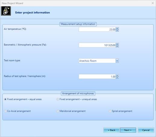
Crystal Instruments has developed software compliant with the ISO 3744:1994 and ISO 3745:2003 standard – Acoustics – Determination of sound power levels of noise sources using sound pressure – Precision methods for anechoic and hemi-anechoic rooms.
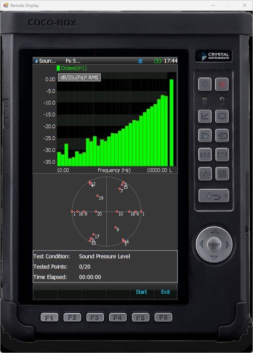
Sound pressure can be measured using any of the Crystal Instruments data acquisition systems. However, accurate analysis requires knowledge of the microphone positions. Fortunately, the CoCo systems include dedicated software designed for this purpose, allowing users to define key factors such as microphone geometry, environmental conditions, and test room type.

Alternatively, the Spider systems or the GRS can be used to acquire sound pressure measurements. Afterwards, users can input the testing parameters and measurement locations into Post Analyzer software.
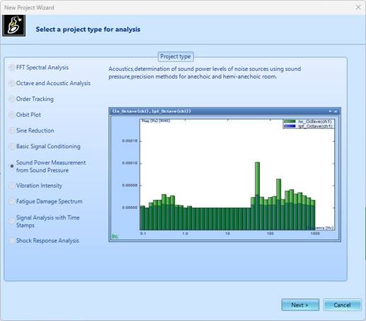
The Post Analyzer software requires two signals per measurement point: a 1/3 octave spectrum of the active noise source, and a 1/3 octave spectrum of the background noise. Using this information, as well as the geometry of the measurement points and environmental conditions, the software can generate an octave spectrum that represents the sound power flux. The diagram below provides a simplified overview of the signal flow required to determine the sound power.

Sones & Phons
Two sounds with equal intensity do not necessarily have the same ‘loudness’ to humans. Loudness is a subjective term used to describe the human ear’s perception of the strength of a sound. Sones and phons are used to quantify the loudness of a sound.
- A phon is a logarithmic unit of loudness. The number of phons of a sound is defined as the sound pressure level, in decibels, of a 1000 Hz tone that would be perceived to be equally as loud as the sound being measured.
- If a sound is perceived to be as loud as 40 dB at 1000 Hz then it is said to have a loudness of 40 phons.
To better understand this concept, Equal Loudness Curves provide an excellent visual representation of how tones with different frequencies and intensities can be perceived as equally loud. The plot below displays the set of contours, which indicate the sound pressure levels required for tones at different frequencies to be perceived as equally loud by the human ear.

A sone is a unit of loudness derived from the number of phons of a sound. Typically, 40 phons are equivalent to 1 sone, and from this point forward every increase of 10 phons is equivalent to doubling the number of sones.
One sone is equivalent to 40 phons, 2 sones is equivalent to 50 phons, 4 sones is equivalent to 60 phons, etc.
Both the Dynamic Signal Analyzer software and the Post Analyzer software can facilitate the conversion of an octave spectrum of sound pressure into a display that represents the sound level in phons or sones. The process is made effortless through the software’s user-friendly interface.
Noise Criterion
Noise criteria curves are commonly used to characterize background noise in buildings and spaces. The curves were developed to ensure that the sound levels in indoor spaces are safe, comfortable, and appropriate for their intended use. There are multiple noise curves because the acceptable amount of sound pressure varies depending on the type of room. The table below serves as a guideline for selecting the appropriate noise curve to use when evaluating the sound level of a room.

Noise criteria are calculated by measuring the background noise in a building using a 1/1 octave spectrum ranging from 63 Hz to 8000 Hz. The curves can be superimposed on an octave spectrum in the Dynamic Signal Analyzer or Post Analyzer software. The DSA software allows users to measure and view real-time sound pressure and compare it against the curves.
Acoustic Control
Crystal Instruments provides hardware solutions that not only serve as data acquisition systems but also function as controllers. A simple control system comprises of three main components:
- Input - The reference or target signal.
- Operator (Crystal Instruments Spider system) - The system that acts on the input signal. This can involve processes such as computations, manipulations, or transformations, depending on the application and goal of the control system.
- Output - The result of the operation performed on the input. The output is then routed back to the input of the control system, creating a feedback loop.
Acoustic control encompasses the process of manipulating audios sources based on a predefined frequency spectrum. Building upon the outline of the control system described above, the Spider system functions as the operator in this context. It drives the audio source which serves as the output. A microphone serves as the input and is used to measure the audio output. The microphone, Spider, and audio source combine to form a closed-loop control system.
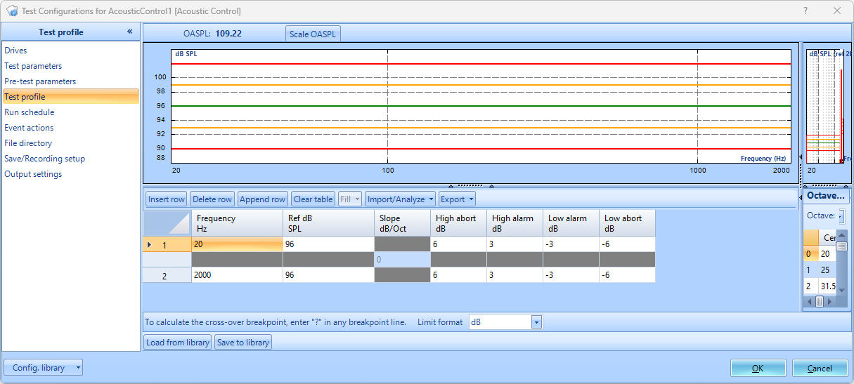
The Vibration Controller software provides users with a customizable acoustic testing option to accommodate any specific needs.
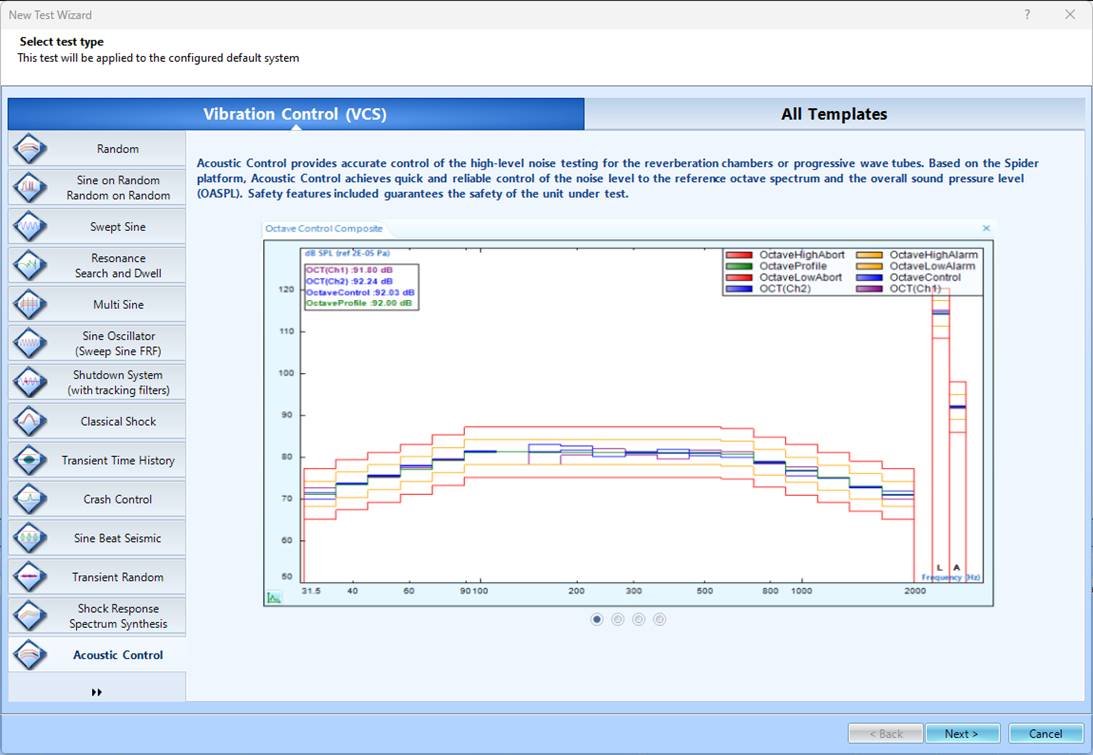
The software offers both single-input-single-output (SISO) and multiple-input-multiple-output (MIMO) control strategies. The predefined frequency spectrum is known as the reference profile and is the target of the control system.

Users can overlay their reference profile with alarm and abort thresholds. In the event that the feedback input signals surpass the alarm limits, a notification will be dispatched. Furthermore, users can configure certain actions to be executed when an alarm is triggered. Exceeding the abort thresholds will invoke the Spider controller to end the test for safety measures.
Microphones for Acoustic Acquisition
Users should carefully choose an appropriate microphone to realize the full capabilities of Crystal Instrument’s data acquisition systems. The quality of acoustic signal analysis, specifically in terms of signal-to-noise ratio and frequency response, relies not only on the data acquisition system but also on the microphone. It is important to recognize these factors which can become potential bottlenecks that impact the overall analysis quality.
Some parameters to consider when selecting a microphone for acoustic measurements:
- Sensitivity – The sensitivity refers to the microphone’s ability to convert sound pressure into voltage. A higher sensitivity is beneficial for accurately capturing low-level sounds.
- Frequency Response – The microphone should ideally have a flat frequency response across the desired measurement range to avoid distortion or attenuation of specific frequencies.
- Signal-to-Noise Ratio – A high SNR ensures that a microphone accurately captures the desired sound while minimizing the background noise.
- Directionality – Omnidirectional microphones capture sound from all directions whereas directional microphones focus on specific angles. The appropriate directionality is based on the desired sound source isolation and application.
- Environmental Considerations – In certain scenarios, a microphone necessitates the ability to endure environmental factors such as temperature, humidity, dust & debris etc.
The GRS is specifically designed to remotely measure sound pressure in harsh environmental conditions. For this reason, we recommend a G.R.A.S. ½” LEMO free-field microphone since it can withstand a large temperature and humidity range. Additionally, the microphone would be placed into an enclosure for protection against rain, dust, and debris.


Crystal Instrument’s DAQ systems are compatible with a wide range of microphones. A notable advantage of our systems is their ability to seamlessly read TEDS (Transducer Electronic Data Sheet) data. This convenient feature eliminates the need for users to manually input sensor parameters. The table below below presents the minimum and maximum sound pressure levels that can be measured using the GRS with different types of commonly used microphones.
| GRS Measurement Range with Various Microphones | |||
|---|---|---|---|
| Microphone Model | Sensitivity | Minimum SPL(A) | Maximum SPL(A) |
| PCB 378A12 | 0.25 mV/Pa | 60 dB | 182 dB |
| PCB 376A31 | 2 mV/Pa | 40 dB | 165 dB |
| PCB 378M12 | 10 mV/Pa | 26 dB | 159 dB |
| PCB 376A32 | 50 mV/Pa | 15.5 dB | 137 dB |
| GRAS 46AC | 12.5 mV/Pa | 20 dB | 164 dB |
| GRAS 46AZ | 50 mV/Pa | 17 dB | 138 dB |