
Modal Testing Excitation Consideration
Download PDF | Jeff Zhao, Ph.D. - Senior Product Manager | © Copyright Crystal Instruments 2018, All Rights Reserved.Contents: 1. Overview | 2. Hammer Impact Testing | 3. Modal Shaker Testing
1. Overview
There are several modal testing methods that consider different types of excitations used. Commonly known methods include Hammer Impact testing and Modal Shaker testing. Please note that Operational Modal Analysis utilizing Ambient Excitation will not be discussed here.
Hammer impact testing uses an Impact Hammer to excite the structure under test. The impulse force applied to the structure is categorized in the broadband range excitation because it contains energy up to a certain frequency range. The hammer impact test is quick to set up and to carry out, and thus is widely used. However, it does have its limitations and there are some concerns to be considered.
Modal shaker testing utilizes a modal shaker to excite the structure under test. Users can select from a list of waveform types to excite the structure under test. This testing method is usually applied to complex or large scale structural testing. Compared to the hammer impact test, it is easier to duplicate. On the other hand, the modal shaker testing method requires more hardware (i.e., modal shaker(s), stinger, more input and output channels from the dynamic signal analyzer). This test setup requires an experienced user.
Ambient excitation uses the natural excitation of the structure, which results in response-only measurement data. This can be used for testing on bridges, buildings, and more in the civil engineering field. This method does not require any boundary condition set-ups and excitation equipment is not required. Since the excitation is unknown, unscaled modal data will be the result. The analysis will require special processing.
2. Hammer Impact Testing
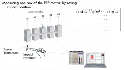
When using an impact hammer to run modal testing, there are two ways to perform the measurement. One method includes a roving hammer with a fixed response measurement point and an excitation point roving over the measurement DOFs on the structure under test. The FRF signals between the fixed response measurement DOF and excitation DOFs are acquired. This results in one row of FRF signals.
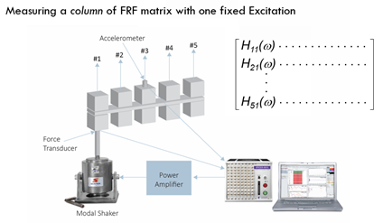
Equivalently, the roving response method can be used. The responses can be measured at several DOFs, while the excitation is fixed at one DOF on the structure under test. With this arrangement, a column of FRF signals will be acquired. With possible multiple responses measured simultaneously, a large amount of FRF signals can be measured at the same time. This will speed up the testing process. However, this will result in the so-called mass loading issue due to the response accelerometers moving from one batch of measurement points and direction to the next. To address this issue, either dummy blocks can be applied to all DOFs are not under measurement; or ultimately make use of enough accelerometers to measure all DOFs in one shot.
The structure under test varies from case to case, which creates a requirement for different hammer sizes to be used. Vendors of testing equipment typically provide hammers in varying sizes, from the mini hammer for PCB board testing to the large sledge hammer for huge rotor testing at power plants.
The hammer tip or its material plays a big role in considering the upper frequency the test will require. The softer hammer tip will result in a relatively lower level impact with a wider width of time. From the frequency domain, the auto power spectrum of the impact pulse decays faster with the use of a harder hammer tip. The following graph illustrates this in the time and frequency domain. It is advisable to choose a hammer tip material with an auto spectrum decay that is less than 6 dB from the upper frequency of the setup.
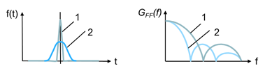
Soft (2) vs hard (1) tip of the hammer
To alleviate leakage, apply the Force/Exponential window as shown below.
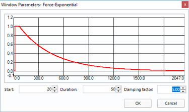
Force/Exponential window with setup parameters
With the application of this window, the response channel data can decay to zero as shown in following graphs.
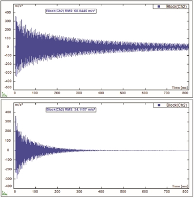
Response signal after Force/Exponential window
Although the Force/Exponential window assists with the leakage issue, it ends up introducing extra damping to the result. Technically, the extra damping introduced can be extracted after the modal results are identified. If it is possible, increase the block size first to allow increased measurement time so that the responses from the structure under test can decay close to a zero level. If this is the case, then no Force/Exponential window will need to be applied.
Double hit is a very common phenomenon that occurs during hammer impact testing. It tends to occur more easily when the hammer hits the edge of a structure. During the occurrence, the spectrum of the excitation will be distorted, thus causing the measured FRF signal to become distorted as well. As a result, the current set of data will be discarded. Many modal software manufacturers implement the double hit detection and auto reject feature in their products. With this feature turned on, the data can be rejected automatically when a double hit is detected.
The driving point defines the measurement for the response DOF, which is the same as the excitation DOF. It can be used to help select the fixed driving point DOF for a roving response hammer test or the fixed response point DOF for a roving excitation hammer test. The process begins with selecting select several DOFs on the mesh of the structure under test. Then a test to measure the FRF will be performed. Check the FRF signals from the driving point selection process to choose a driving point from the FRF illustrating the most resonance peaks and the valley existing between any two resonances. This is accomplished with a hammer impact test, but the result is applicable for modal shaker tests as well. The selected DOF can be applied for a modal shaker test to attach a driving stinger onto a modal shaker.
3. Modal Shaker Testing
Modal Shaker Excitation testing involves exciting the structure at one fixed DOF and measuring DOFs as the number of responses. FRF signals between the response DOFs and excitation DOF are computed., One column of FRF signals are measured with single input (excitation) multiple output (response). When the input channel count of the Dynamic Signal Analyzer is not high enough to cover all the measurement DOFs in one shot, the measurement sensors can be roved, and the measurements can be repeated to finish all the required response DOFs.
An output channel on the Dynamic Signal Analyzer will be used to drive the amplifier of the modal shaker. Many waveform types are available to drive the structure under test. A common choice to drive the structure under test is Pure Random (Gaussian Random, or White Noise). Due to the nature of leakage, a window (such as a Hann window), needs to be applied with this type of excitation waveform.
Another commonly used excitation waveform for Modal shaker testing is Burst Random. This signal type is still categorized as random; it generates a random signal with a user defined percentage while not sending a drive out. This allows the structural response to decay within the zero-output duration of each block of data. In case the response does not decay enough, the percent of burst random can be tuned to increase the zero-output period. With this in place, there will be no leakage and thus no windowing would be required. This is the main reason for selecting Burst Random excitation.
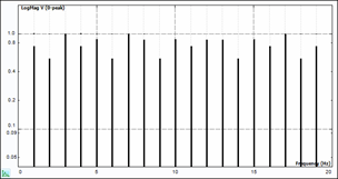
Periodic Random and Pseudo Random are more categories of random waveforms. Pseudo Random is defined as an ergodic, stationary random signal consisting of energy content only at integer multiples of the FFT frequency lines (Δf). The linear spectrum of this signal is shaped to have a constant amplitude, but with random phase. The following figure illustrates the constant amplitude characteristics of the pseudo random signal.

Pseudo Random Signal Spectrum
When sufficient time delay is allowed during the measurement procedure, any transient response to the initiation of the signal will decay, and the resulting input and output blocks are periodic with respect to the sampled period (block size).
The Periodic Random signal is also an ergodic, stationary random signal consisting only of integer multiples of the FFT frequency increment. The frequency spectrum of this signal has random amplitude and random phase distribution. The following figure illustrates the spectrum characteristics.
Periodic Random Signal Spectrum
For each spectral average, an input signal is generated with random amplitude and random phase. The system is excited with these multiple input blocks, until the transient response to the change in the excitation signal decays. The input and response histories should then be periodic with respect to the block-size and should be saved as one spectra average in the total process. With each new average, a new block of signals, random with respect to previous input signals, is generated so that the resulting measurement will be completely randomized.
Sine excitation waveforms are also available, i.e., Chirp, Burst Chirp.
Periodically multiple excitation testing is required, which is referred to as Multiple Input Multiple Output (MIMO) testing. This method is usually implemented for large and supple structures’ modal testing. With the use of multiple modal shakers, the excitation energy will be sufficiently distributed to excite the global modes of the structure under test. Simply increasing the driving force with a single shaker arrangement will overstress the driving point and cause nonlinearity in the behavior of the structure.
For structures with repeated modes, or highly coupled modes, MIMO modal testing will result in multiple columns of FRF. With this information, the repeated modes or highly coupled modes can be identified by using the corresponding FRF matrix. It should be noted that the parameter identification method to handle the poly-reference FRF matrix is also categorized as poly-reference. With an identified mode participation factor, the repeated or highly coupled modes can be isolated.