
Advanced Patented Methodologies in Ground Vibration Testing for Aerospace Applications
DOWNLOAD PAPER | ABSTRACT
To ensure aircraft safety and flutter-free operation within safe flight envelopes, high-channel-count Ground Vibration Testing (GVT) systems are widely employed for structural analysis. These systems facilitate seamless data acquisition, analysis, and post-processing to assess the dynamic behavior of aircraft. However, traditional GVT approaches often involve extensive cabling, complex test setups, and time-intensive data processing, making them cumbersome and resource-intensive.
Leveraging patented vibration visualization technology, an innovative solution is developed that interpolates data from hundreds of measurement points to thousands of geometric points, enhancing spatial resolution and test accuracy. The GVT modal test integrates multiple modal shakers generating burst random excitations while simultaneously collecting response data from hundreds of accelerometers. The system efficiently processes large datasets of Frequency Response Functions (FRFs) into simplified mode indicator functions and employs frequency-domain curve fitting to extract critical parameters, including natural frequencies, damping ratios, and mode shapes.
This paper presents an experimental case study showcasing the application of this patented technology on a fighter jet, demonstrating its effectiveness in aerospace, defense, commercial, and UAV platforms. The results highlight the efficiency and precision of this advanced methodology in structural dynamic testing.
Keywords: Ground Vibration Testing, Patented Vibration Visualization, Aerospace, Fighter Jet, Experimental Modal Test, Dynamic Properties
INTRODUCTION
Ground Vibration Testing (GVT) is a fundamental technique in aerospace structural dynamics, providing critical insights into an aircraft's response to vibrational excitations. This method allows engineers to determine key modal properties—natural frequencies, damping ratios, and mode shapes—essential for ensuring the structural integrity, flutter resistance, and overall safety of an aircraft throughout its operational life.

Fig.1 Basic Workflow of GVT Modal Test on aircraft assembly and its sub-components
Traditional GVT methods rely on high-channel-count measurement systems to capture dynamic responses. However, these approaches are often constrained by limited sensor density, making it difficult to achieve a fully detailed visualization of mode shapes. The reliance on extensive sensor networks and complex wiring increases operational costs, setup time, and data processing challenges. These limitations present several key issues:
Sparse Measurement Grids: Limited sensor placement results in gaps in mode shape visualization, reducing the accuracy of structural assessments.
High Operational Costs: Large-scale testing demands extensive sensor deployment and significant manual labor, increasing both cost and complexity.
Data Correlation Challenges: Missing measurements at non-instrumented points create difficulties in aligning experimental results with numerical simulations, affecting model validation.

Fig.2 Cabling issues with traditional approach
To address these challenges, this study presents an advanced interpolation-based technique that significantly enhances the spatial resolution of mode shape representation. By leveraging a refined 3D geometric model and interpolating between measured and unmeasured points, this method enables a more comprehensive visualization of deformation patterns without requiring additional hardware resources. This approach effectively bridges gaps in modal measurements, improving the accuracy of structural assessments while optimizing both time and cost constraints.
The proposed methodology not only refines GVT but also streamlines the overall testing process by reducing reliance on extensive sensor deployments. The following sections provide a detailed analysis of this technique, demonstrating its effectiveness in advancing aerospace structural testing. By integrating innovative spatial resolution enhancement methods, this approach improves both efficiency and accuracy in modal analysis, offering a scalable and cost-effective solution for aerospace applications. Furthermore, the patented interpolation technique is adaptable to spaceflight and spacecraft structures, even those with intricate geometries across three dimensions.
EXPERIMENTAL WORKFLOW
An experimental GVT was conducted on a fighter jet to evaluate the proposed mode shape interpolation methodology. This approach integrates conventional GVT modal testing with an advanced vibration visualization technique to enhance the spatial resolution of mode shapes while optimizing data acquisition and analysis efficiency.
The process begins with the import of a detailed 3D geometric model of the aircraft, ensuring accurate representation of its structural framework. Measurement points are strategically assigned across critical structural components, serving as the basis for data acquisition. Input channel setup is then configured, defining sensor locations and data acquisition parameters. Output channel configuration follows, ensuring proper excitation settings and response logging for the modal test.
During measurement execution, excitation forces are applied to the aircraft using modal shakers, while accelerometers record the dynamic response. The acquired raw vibration data is then processed through a structured workflow. Modal data selection is performed to extract relevant response signals, followed by the application of a mode indicator function to identify dominant modal characteristics. Curve-fitting techniques, such as the Poly-X algorithm, are employed to refine modal parameter estimation, including natural frequencies and damping ratios.
Finally, the mode shape interpolation technique is applied to enhance the spatial resolution of modal results. By leveraging interpolation across measured and non-measured points, this approach provides a comprehensive visualization of the aircraft’s deformation patterns.

Fig.3 Experimental Workflow Chart
This methodology demonstrates the effectiveness of interpolation-based vibration visualization in GVT, offering a cost-effective and efficient solution for aerospace structural testing. The results highlight the potential for broader application in aircraft and spacecraft modal analysis.
1. Geometric Modeling and Measurement Layout
The first critical step in this modal analysis workflow involves strategically assigning measurement points across the aircraft's wingspan and mapping them onto a detailed 3D geometric model. This geometric model, imported into the analysis software, serves as the reference framework for vibration testing. A total of 28 measurement points is distributed across key structural locations, ensuring comprehensive coverage of the aircraft’s dynamic response.

Fig.4 Measurement points chosen on imported 3D model

Fig.5 Measurement grid laid out on the aircraft
Once the measurement grid is established, sensors are placed at these predefined points to capture vibration data during GVT. The data collected from these measurement locations is later utilized in an interpolation technique to estimate responses at unmeasured points, thereby improving spatial resolution without requiring additional hardware. This methodology allows for a more complete and precise visualization of the mode shapes, enhancing the accuracy of structural analysis while optimizing test efficiency.
2. Input Channel Setup
The second step in the process involves mapping excitation and response channels according to the experimental setup. To ensure precise excitation and response measurement, a fixed modal shaker is strategically placed to introduce controlled vibrations into the aircraft structure. This excitation allows for the accurate capture of structural responses under known input conditions.

Fig.6 Uni-axial accelerometers placed on measurement points
For response measurements, seven uni-axial accelerometers are roved across designated measurement points on the aircraft's wings. These sensors record acceleration data, enabling the characterization of the aircraft’s dynamic behavior. The measured responses are systematically logged and assigned in the channel configuration, as shown in the channel table.
Due to limitations of the test system, acceleration data from the impedance head—typically used for drive point measurements in GVT—is not acquired. Additionally, only out-of-plane acceleration data is recorded for the same reason. Nonetheless, the interpolation technique applied in this study is adaptable to full 3D measurement datasets.

Fig.7 Input channel setup
This setup ensures that sufficient data is collected across the aircraft to support accurate modal parameter estimation. The acquired response data will be further processed through mode shape interpolation, enhancing the spatial resolution of modal analysis without increasing sensor density.
3. Output Channel Setup
In the next step, the output channel is configured to drive the modal shaker, ensuring controlled excitation of the aircraft. The modal shaker is securely mounted beneath the wing, with force applied through a stinger attachment to introduce vibrations into the airframe. This setup is critical for accurately exciting the structure while minimizing any unintended constraints on the system.

Fig.8 Modal shaker mounted on desired measurement point
To optimize excitation and prevent spectral leakage, a Burst Random signal is employed, with an 80% burst rate applied through the output channel configuration. This technique ensures that the excitation remains within the desired frequency range while avoiding interference from overlapping signal windows. The configuration parameters, including amplitude and burst rate, are defined in the output channel settings and verified through the real-time signal preview.

Fig.9 Output channel setup
By implementing this precise excitation strategy, the test ensures that modal parameters—such as natural frequencies, damping ratios, and mode shapes—are accurately captured for further analysis. This controlled approach enhances the reliability of the measured data while facilitating efficient extraction of structural dynamic characteristics.
4. FFT and Correction
In GVT, accurate modal analysis relies on transforming time-domain vibration signals into the frequency domain to extract key dynamic properties. This transformation is achieved through the Fast Fourier Transform (FFT), which converts measured acceleration and excitation signals into the frequency domain:
Fj(ω) = F{fj (t)}
- fj(t) is the input excitation force
- Fj(ω) is the converted spectral representation
Xi(ω) = F{xi (t)}
- xi(t) is the measured structural response
- Xi(ω) is the converted spectral representation
To establish meaningful relationships between input and response signals, the Cross Power Spectral Density (CPS) and Auto Power Spectral Density (APS) are computed:


 is the cross-power spectral density between measured response Xi (ω) and Fj (ω)
 is the auto-power spectral density of the excitation signal spectral representation
The Frequency Response Function (FRF) is then derived as:

which characterizes how the structure responds dynamically to an applied force across different frequency ranges.
To improve accuracy and minimize noise artifacts, multiple FRF measurements average over N measurement runs:

Averaging helps in reducing experimental variability, improving the reliability of extracted modal parameters such as natural frequencies, damping ratios, and mode shapes.
A crucial metric in validating measurement accuracy is the coherence function (COH), which quantifies the consistency of the input-output relationship across multiple test runs:

where  ranges from 0 to 1, with values close to 1 indicating a strong linear relationship between input and output signals, signifying high measurement quality. A lower coherence value suggests potential noise, nonlinearities, or poor excitation levels, requiring careful examination.

Fig.10 GVT Modal Measurement
For this GVT modal test, the lower order modes are of interest and therefore a sampling rate of 100 Hz is set. A block size of 1024 is selected. A fine frequency resolution of 0.097 Hz is produced with these configuration settings. Measurements of higher accuracy and reduced noise are obtained by linearly averaging 8 blocks of data at each measurement DOF.
Burst random excitation imparts energy across a broad frequency range of 45 Hz and has the added advantage of user tunable burst percentage to control the no output duration time which allows the responses to decay to zero. With this setup, there will be no leakage, and uniform window can be selected. For this test, the output amplitude was set to 1V with an 80% burst rate.
The 80% burst rate ensures that the shaker provides excitation for 10.24 seconds in each time block and there is no output for the remaining 2.048 seconds. This information is graphically represented in the plot shown above.
The coherence plot is acceptable. The valleys in the coherence plot occur at the anti-resonances which indicate that the response level is relatively lower at these corresponding frequencies. So overall, the inputs and outputs are well correlated in the desirable frequency range.
5. Modal Data Selection
After the FRFs are computed for each measurement point, they are analyzed collectively to identify dominant peaks and ensure modal consistency. FRFs describe the relationship between input forces and measured responses across multiple locations, forming an FRF matrix:

where Hij represents the transfer function between the i-th excitation point and the j-th response measurement.

Fig.11 Modal Data Selection
To ensure accuracy, 28 compatible FRFs are selected, corresponding to the 28 measurement locations on the aircraft structure. These FRFs are overlaid to compare dominant peaks, which indicate the natural frequencies of the aircraft. Peaks in the FRF correspond to modal resonances, where the aircraft exhibits maximum response under vibrational excitation. By analyzing these resonances, engineers can extract critical modal parameters such as natural frequencies, damping ratios, and mode shapes.
6. Mode Indicator Function
The Complex Mode Indicator Function (CMIF) is a powerful tool used in modal analysis to identify the natural frequencies and modes of a structure. It is particularly effective when applied to the FRF matrix obtained from GVT, where multiple output measurements are taken under controlled excitation.
With the steps described above, multiple measurements are taken across different points on a structure to capture its vibrational response. The FRF matrix Hij is a collection of frequency response functions between response and excitation signals.
The CMIF is derived by performing Singular Value Decomposition (SVD) on the FRF matrix for each frequency bin K. The SVD decomposes the FRF matrix as follows:
Hij[K] = U[K]Σ[K]VH[K]
- U[K] and V[K] are unitary matrices representing the left and right singular vectors, respectively
- Σ[K] is a diagonal matrix containing the singular values σ1 [K],σ2 [K],…,σr [K] at a given frequency bin K
- VH[K]is the Hermitian transpose of V[K]

Fig.12 CMIF plot indicating modes from the FRF matrix
The CMIF is defined as the plot of the singular values σi[K] across all frequency bins K. The peaks of these singular value curves indicate the presence of modes, as they correspond to frequencies at which the structure exhibits strong vibrational energy.
CMIF[K] = Max(σ1[K],σ2 [K],…,σr[K])
The use of CMIF, derived from SVD, helps separate true modes from noise and artifacts in the data. CMIF can simultaneously highlight multiple modes present in the structure. The function provides a clear and intuitive method for identifying natural frequencies by visually analyzing singular value peaks.
7. Modal Parameter Extraction
Curve-fitting is the process of applying mathematical models to data points to identify specific characteristics—in this case, the modal parameters of an aircraft from the CMIF data. The Poly-X method is a sophisticated algorithm used to fit the CMIF data to extract these modal parameters, such as natural frequencies, damping ratios, and mode shapes.
The Poly-X method, also known as the Poly-reference least-squares complex frequency-domain (p-LSCF) method, is a high-resolution technique for curve-fitting frequency response functions. It is particularly effective for experimental modal analysis due to its robustness in handling noise and complex systems.
In the p-LSCF method, the system's response in the frequency domain is represented using a polynomial model. This model relates the response outputs to a known input which is inherent in EMA.
The characteristic polynomials N(z) & D(z)is used to express the system's behavior, where z is a complex exponential representing the discrete frequency variable:
z=ⅇjωT
-
ω is the angular frequency
-
T is the sampling period of the data
The polynomial D(z)is expressed as
D(z)=1+d1 z-1+d2 z-2+⋯+dn z-n
This polynomial has coefficients di that are determined through the curve-fitting process.
The goal of curve-fitting in the p-LSCF method is to find the polynomial D(z) such that the roots (or poles) of this polynomial match the dynamics observed in the FRF matrix. The FRF matrix Hij (ω)contains frequency response function information that reflects the relations between the responses and excitation at various points on the structure. By fitting a polynomial model to this matrix across frequency bins, we can identify the frequencies at which the structure has significant vibrational energy, corresponding to the natural frequencies.
The curve-fitting step involves minimizing the difference between the polynomial representation of the system and the actual FRF data. This is done by solving a least-squares problem:
 is the modeled FRF data based on the polynomial
- M is the number of frequency bins
To perform this curve-fitting, the least-squares approach is used to find the coefficients d1,d2,…,dn of the polynomial D(z). These coefficients define the polynomial that best fits the FRF data over the frequency range analyzed. The fitting process can be visualized as finding the set of coefficients that minimizes the error between the actual FRF matrix values and the values predicted by the polynomial model.
After the polynomial D(z) is determined, its roots (poles) are calculated:

Where zi are the complex roots of the polynomial. The locations of these poles in the complex plane reveal the modal properties:
- The frequency of the mode which can be represented as
The damping ratio of the mode which can be represented as

The results of the curve-fitting process are displayed in a stability diagram, where the poles identified across different model orders are plotted.
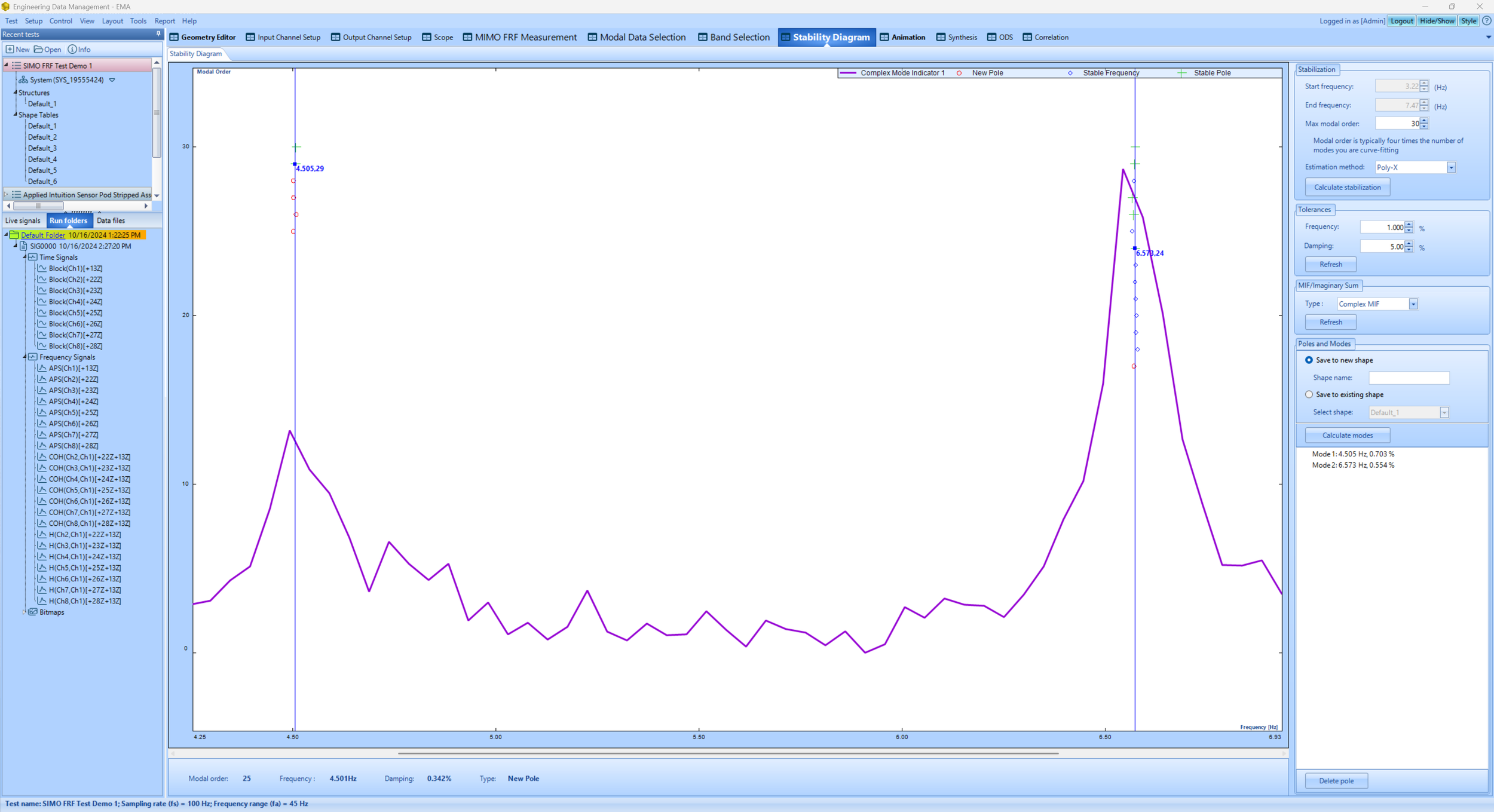
Fig.13 Poly-X Stability Diagram
Poles that consistently appear in multiple model orders are considered true modes, while others that vary significantly are treated as noise or computational artifacts.
8. Modal Shape Extraction and Interpolation
Through FRF matrix decomposition, SVD, and curve-fitting techniques, we ensure that modal parameters such as natural frequencies, damping ratios, and mode shapes are accurately captured, providing a reliable representation of the aircraft’s dynamic behavior. Furthermore, the interpolation technique enhances mode shape visualization, enabling better correlation with Finite Element Models (FEM) while reducing sensor requirements and improving testing efficiency.
The FRF matrix H(ω)is expressed as a summation of modal contributions.
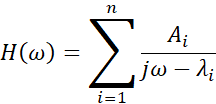
- Ai is the residue matrix which captures the influence of each mode
- λi = σi + jωi are the complex modal poles
The residue matrix Ai is computed as
Ai = (jω - λi)H(ω)
SVD is applied to this residue matrix Ai
Ai = Ui ΣiViT
- Ui contains the left singular vectors, representing mode shapes.
- Σi contains singular values, indicating mode significance
- ViT contains the right singular vectors
To ensure consistency in mode shape representation, normalization is performed using the maximum absolute value:

This ensures that the largest value of each mode shape is scaled to unity, making comparisons between different modes and test conditions easier.
To assess the correlation between extracted mode shapes, the Modal Assurance Criterion (MAC) is used. MAC provides a numerical measure of similarity between two mode shapes Φi and Φj

A MAC value close to 1 indicates a high correlation (similar mode shapes). A MAC value near 0 suggests that the two mode shapes are significantly different.
Using the mode shape data at measurement locations, the deformation vectors at unmeasured locations is computed as:

- DA is the interpolated deformation at the unmeasured point.
- Di represents the measured deformation at point i
- wi is the interpolation weight assigned to each measured point.
- N is the total number of measured points contributing to the interpolation.
The interpolation weights are determined based on the distance between measured and unmeasured points. A common approach is inverse distance weighting (IDW), which assigns greater weight to closer points:

- ⅆi is the Euclidean distance between the unmeasured point and the measured point i
 ensures that the sum of weights is normalized to 1, preventing scaling inconsistencies.
In this approach, the closer points contribute more to the interpolated value and distant points have a reduced influence.

Fig.14 Modal Parameters of fighter jet

Fig.15 Bending mode of the fighter jet at 6.562 Hz
First Bending Mode at 6.562 Hz: Representing lateral displacement.

Fig.16 Torsion mode of the fighter jet at 12.976 Hz
First Torsion Mode at 12.976 Hz: Indicating torsional response.
Interpolating mode shapes over unmeasured points offers several benefits in aerospace structural testing:
Enhanced Spatial Resolution – Provides a continuous mode shape visualization across the structure.
Reduced Sensor Requirements – Enables accurate deformation estimation with fewer physical sensors.
Improved Correlation with FEM Models – Finer mode shape mapping enhances Finite Element Model (FEM) validation.
The analysis of the FRF matrix through SVD, and curve-fitting forms the backbone of modal analysis in EMA. The application of these techniques ensures that the extracted natural frequencies, damping ratios, and mode shapes are reliable and representative of the aircraft’s actual dynamic behavior.
Additionally, the interpolation technique enhances mode shape visualization by providing a more detailed and continuous representation of structural deformation without requiring additional physical sensors. This not only improves the clarity of mode animations but also significantly reduces testing time and costs, making modal analysis more efficient and scalable.
These results demonstrate the importance of precise modal data extraction, which is essential for aircraft and spacecraft structural analysis, flutter prediction, and aerospace safety assessments.
CONCLUSIONS AND FUTURE DIRECTIONS
This study successfully validated the efficiency and reliability of interpolation techniques in Ground Vibration Testing (GVT), demonstrating their ability to accurately identify modal properties while minimizing the need for extensive wiring and reducing costs. This marks a significant advancement in aerospace structural testing, enabling more efficient and scalable modal analysis.
Future research could extend this methodology to more complex structures, such as spacecraft, where accurate modal characterization is critical. Additionally, the interpolation technique holds potential for real-time and offline animation of time-domain and spectral data, enhancing vibration analysis and structural monitoring in intricate aerospace systems.


Fig.17 Pictorial illustration of an EMA test on a Satellite with some results


Fig.18 Illustration of a Realtime & Offline animation of time & spectrum data on aircrafts with some results
REFERENCES
1. Inman, Daniel J., “Engineering Vibrations, Second Edition,” Prentice Hall, New Jersey, 2001.
2. Bart Cauberghe et al. “The secret behind clear stabilization diagrams: the influence of the parameter constraint on the stability of the poles”. In: Proceedings of the 10th SEM international congress exposition on experimental and applied mechanics. 2004, pp. 7–10.
3. Sanjit K. Mitra and James F. Kaiser, Ed. Handbook for Digital Signal Processing, Wiley-Interscience, New York, 1993.
4. James Zhuge, Weijie Zhao, Aakash Umesh Mange, US Patent #11,287,351, granted on 3/29/2022, Vibration Visualization with Real-Time and Interpolation Features.
5. Aakash Umesh Mange, James Zhuge, “Obtain Vibration Mode using GPS Technology”, Crystal Instruments, 2024.