
Basics of Structural Vibration Testing and Analysis
Download PDF | by Jeff Zhao, Ph.D. - Crystal Instruments Senior Product Manager | © Copyright Crystal Instruments 2016, All Rights Reserved.Contents: 1. Section One | 2. Section Two | 3. Section Three | 4. Section Four
Section 1
Introduction
Structural vibration testing and analysis contributes to progress in many industries, including aerospace, auto-making, manufacturing, wood and paper production, power generation, defense, consumer electronics, telecommunications and transportation. The most common application is identification and suppression of unwanted vibration to improve product quality.
This application note provides an introduction to the basic concepts of structural vibration. It presents the fundamentals and definitions in terms of the basic concepts. It also discusses practical applications and provides real world examples.
This paper covers the following topics:
- Basic terminology
- Models of single and multiple degree of freedom
- Continuous structure models
- Measurement techniques and instrumentation
- Vibration suppression methods
- Modal analysis
- Operating deflection shape analysis
Basic Terminology of Structural Vibration
The term vibration describes repetitive motion that can be measured and observed in a structure. Unwanted vibration can cause fatigue or degrade the performance of the structure. Therefore it is desirable to eliminate or reduce the effects of vibration. In other cases, vibration is unavoidable or even desirable. In this case, the goal may be to understand the effect on the structure, or to control or modify the vibration, or to isolate it from the structure and minimize structural response.
Vibration analysis is divided into sub-categories such as free vs. forced vibration, sinusoidal vs. random vibration, and linear vs. rotational vibration.
Free vibration is the natural response of a structure to some impact or displacement. The response is completely determined by the properties of the structure, and its vibration can be understood by examining the structure's mechanical properties. For example, when you pluck a string of a guitar, it vibrates at the tuned frequency and generates the desired sound. The frequency of the tone is a function of the tension in the string and is not related to the plucking technique.
Forced vibration is the response of a structure to a continuous forcing function that causes the structure to vibrate at the frequency of the excitation. For example, the rear view mirror on a car will always vibrate at the frequency associated with the engine's RPMs. In forced vibration, there is a deterministic relationship between the amplitude of the corresponding vibration level and the forcing function. The relationship is dictated by the characteristics of the structure.
Sinusoidal vibration is a special type of vibration. The structure is excited by a forcing function that is a pure tone with a single frequency. Sinusoidal vibration is not very common in nature, but it provides an excellent engineering tool that enables us to understand complex vibrations by breaking them down into simple, one-tone vibrations. The motion of any point on the structure can be described as a sinusoidal function of time as shown in Figure 1 (top).
Random vibration is very common in nature. The vibration a driver feels when driving a car results from a complex combination of sources, including rough road surface, engine vibration, wind buffeting the car's exterior, etc. Instead of trying to quantify each of these effects, they are commonly described by using statistical parameters. Random vibration quantifies the average vibration level over time across a frequency spectrum. Figure 1 (bottom) shows a typical random vibration versus time plot.
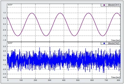
Figure 1. Sinusoidal vibration (top) and random vibration (bottom).
Rotating imbalance is another common source of vibration. The rotation of an unbalanced machine part can cause the whole rotating machine to vibrate. The imbalance generates the forcing function that affects the structure. Examples include a washing machine, an automobile engine, shaft system, steam or gas turbines, and computer disk drive. Rotational vibration is usually harmful and unwanted, and the way to eliminate or minimize it is to properly balance the rotating part of the machine.
The common element in all these categories of vibration is that the structure responds with some repetitive motion that is related to its mechanical properties. By understanding the basic structural models, measurement and analysis techniques, it is possible to successfully characterize and treat vibration in structures.
Time and Frequency Analysis
Structural vibration can be measured by using electronic sensors that convert vibration motion into electrical signals. By analyzing the electrical signals, the nature of the vibration can be understood. Signal analysis is generally divided into time and frequency domains; each domain provides a different view and insight into the nature of the vibration.
Time domain analysis starts by analyzing the signal as a function of time. An oscilloscope, data acquisition device, or dynamic signal analyzer can be used to acquire the signal. Figure 2 illustrates a structure model, such as a single-story building, responding to an impact of vibration that is measured at point A and plotted versus time. The dashed lines indicate the motion of the structure as it vibrates about its equilibrium point.

Figure 2. Mechanical structure responds with vibration plotted versus time.
The plot of vibration versus time provides information that helps characterize the behavior of the structure. Its behavior can be characterized by measuring the maximum vibration (or peak) level, or finding the period (time between zero crossings), or estimating the decay rate (the amount of time for the envelope to decay to near zero). These characteristic parameters are the typical results of time domain analysis.
Frequency analysis also provides valuable information about structural vibration. Any time history signal can be transformed into frequency domain. The most common mathematical technique for transforming time signals into frequency domain is called Fourier Transform, named after the French Mathematician Jean Baptiste Fourier. The mathematical processing involved is complex, but today's dynamic signal analyzers race through it automatically in real-time.
Fourier Transform theory states that any periodic signal can be represented by a series of pure sine tones. Figure 3 illustrates how a square wave can be constructed by adding up a series of sine waves; each of the sine waves has a frequency that is a multiple of the fundamental frequency of the square wave. The amplitude and phase of each sine tone must be carefully chosen to get just the right waveform shape. When using a limited number of sine waves as in Figure 3, the result resembles a square wave, but the composite waveform is still ragged.

Figure 3. A square wave can be constructed by adding pure sine tones.
As more and more sine waves are added in Figure 4, the result looks more and more like a square-wave.
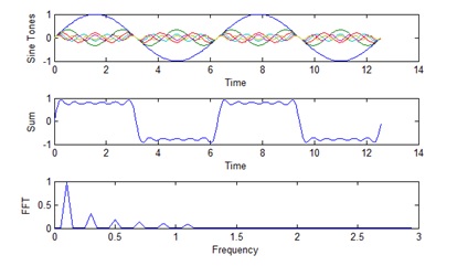
Figure 4. As more sine tones are added the square waveform shape is improved.
In Figures 3 and 4, the third graph shows the amplitude of each sine tones. In Figure 3, there are three sine tones, and they are represented by three peaks in the third plot. The frequency of each tone is represented by the location of each peak on the frequency coordinate in the horizontal axis. The amplitude of each sine tone is represented by the height of each peak on the vertical axis. In Figure 4, there are more peaks as there are more sine tones added together to form the square wave. This third plot can be interpreted as the Fourier Transform of the square wave.
In structural analysis, usually time waveforms are measured and their Fourier Transforms are computed. The Fast Fourier Transform (FFT) is a computationally optimized version of the Fourier Transform. The third plot in Figure 4 also shows the measurement of the square wave with a signal analyzer that computes its Fast Fourier Transform. With testing experience, structural vibration can be understood by studying frequency domain spectrum.
The Decibel dB Scale
Vibration data is often displayed in a logarithmic scale called Decibel (dB) scale. This scale is useful because vibration levels can vary from very small to very large values. When plotting the whole data range on most linear scales, the small signals become virtually invisible. The dB scale solves this problem because it compresses large numbers and expands small numbers. A dB value can be computed from a linear value per following equation,

where xref is a reference number that depends on the type of measurement. Comparing the motion of a mass to the motion of the base, base measurement is used as the reference in the denominator and the mass as the measurement in the numerator.
In dB scale, if the numerator and denominator are equal, the level is zero dB. A level of +6 dB means the numerator is a factor of two times the reference value, and +20 dB means the numerator is a factor of 10 times the reference.
Figure 5 shows an FFT spectrum in linear scale on the top, and dB scale on the bottom. Notice that the peak near 200 Hz is nearly indistinguishable on the linear scale, but very pronounced with the dB scale.
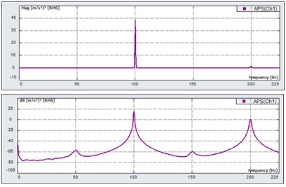
Figure 5. The dB scale allows us to see both large and small numbers on the same scale as shown for the FFT with linear scale on the top and dB scale on the bottom.
Section 2
Structural VibrationStructural vibration can be complex, so let's start with a simple model to derive some basic concepts and build up to more advanced models. The simplest vibration model is the single-degree-of-freedom, or a mass-spring-damper model. It consists of a simple mass (M) that is suspended by an ideal spring with a known stiffness (K), and a dashpot damper from a fixed support. A dashpot damper is like a shock absorber in a car. It produces an opposing force that is proportional to the velocity of the mass.
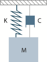
Figure 6. Simple Mass-Spring-Damper Vibration Model
In this model, the factors that affect vibration are completely characterized by the parameters M, K and C. Knowing these values, the structural response to excitation can be predicted exactly.
The mass is a measure of the density and amount of the material. A marble has a small mass and a bowling ball has a relatively larger mass. The stiffness is a measure of how much force the spring will pull when stretched by a given amount. A rubber band has a small stiffness and a car leaf spring has a relatively large stiffness. A sports car with a tight suspension has more damping than a touring car with a soft suspension. When the touring car hits a bump, it oscillates up and down for a longer time than the sports car. Different materials have different damping qualities. Rubber, for example, has much more damping than steel.
If the mass is displaced by pulling down and releasing, the mass will respond with motion similar to Figure 7. The mass will oscillate about the equilibrium point and after every oscillation, the maximum displacement will decrease due to the damper element, till the motion becomes so small that it is undetectable. Eventually the mass element will stop moving.
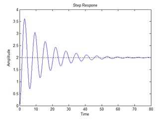
Figure 7. Free Vibration of Mass-Spring-Damper Model
Figure 7 shows that the time between every oscillation is same. The time plot crosses zero at regular intervals. The time for the displacement to cross zero with a positive slope to the next zero crossing with positive slope is named the period. It is also related to the frequency of oscillation.
Frequency can be computed by dividing one by the period value. For the mass-spring-damper model subject to free vibration, the frequency of oscillation is completely determined by the parameters M, K, and C. It is called the natural frequency denoted by the symbol fn. Frequency is measured in cycles per second with units of Hertz (Hz). Assuming the damping is small, then the mathematical relationship is given by

A larger stiffness will result in a higher fn, and a larger mass will result in a lower fn.
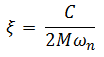
Figure 7 also reveals something about damping. Theory tells us that the amplitude of each oscillation will diminish at a predictable rate. The rate is related to the damping factor C. Usually damping is described in terms of the damping ratio ζ. That ratio is related to C by
The damping ratio can vary from zero to infinity. When it is small (less than about 0.1), the system is lightly damped. When excited, it will oscillate, or ring, for a long time as shown in Figure 8. When the damping ratio is large, the system is 'over damped'. It will not oscillate at all and it may take a long time to return to its equilibrium position. When the damping ratio = 1, the system is 'critically damped' and will return to the equilibrium position in the shortest possible time.

Figure 8. Free vibration of mass-spring-damper for three cases: A - under damped, B - critically damped, C - over damped.
Vibration theory also describes how the mass-spring-damper model will respond to forced vibration. Imagine that the base of the mass-spring-damper is not fixed, but instead forced to move up and down a small distance. If this base motion is sinusoidal, it is straightforward to predict how the mass will respond to the forced vibration. The mass will begin to move in sinusoidal motion at the same frequency as the base; the amplitude of the mass displacement will vary depending on the frequency of the base motion. This is shown in Figure 9 where the mass displacement is larger than the base displacement. There will also be a phase difference between the base and the mass displacement.
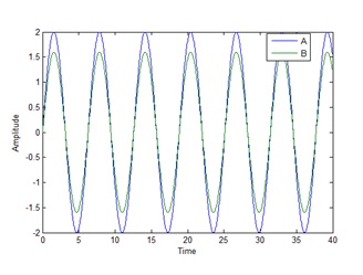
Figure 9. Mass-Spring-Damper Model responds to forced vibration with change in amplitude and phase: A-mass vibration, B-base displacement.
The relative amplitude and phase of the mass displacement will vary with the frequency of the base excitation. Varying the base frequency and recording the corresponding mass displacement amplitude (divided by the base displacement amplitude) and the phase, results in a plot of the vibration amplitude and phase versus excitation frequency.
Figure 10 shows the results for three different values of the damping ratio (ξ). In all cases, the amplitude ratio (Magnitude) is 1 (or zero dB for dB scale) for low frequencies. This means that the amplitudes are equal at low frequencies. As the frequency increases, the magnitude rises to some maximum value. The frequency of this peak is fn, the natural frequency. At frequencies above fn, the magnitude falls of at a constant rate. This plot is known as a Bode Diagram. Note the horizontal axis is of log scale with unit Hz. Note that the peak is higher for light damping. For critical damping (red curve) and over damping (not shown), the magnitude does not increase above 1 (or 0 dB).

Figure 10. Bode Diagram of the vibration of the mass-spring-damper system with A: ζ = 0.1, B: ζ = 0.5, C: ζ = 1
The lower plot in Figure 10 shows the phase relation between the base and the mass for different frequencies. At low frequencies below fn, the phase is zero degrees meaning that the mass is in phase with the base. When the base vibration frequencies coincide with fn (at resonance), the phase is 90 degrees. At high frequencies, the phase is 180 degrees; the mass is out of phase with the base and they move in opposite directions. Note that different damping ratios affect the slope of the phase change.
The Q Factor is a common term used to represent how underdamped an structure is. Vibration theory shows that the damping ratio is related to the sharpness of the peak of the magnitude plot. The damping ratio, ζ, can be determined by computing Q, defined as the resonant frequency divided by the half power bandwidth around the peak at fn. Q factor is computed as:

where fn is the resonant frequency at the peak in Hz; f1 and f2 are the half power points measured -3 dB down from the peak as shown in Figure 11.
Another way to measure damping is to simply record the peak amplitude ratio. However this should not be confused with the Q factor as they are not equivalent.

Figure 11. The Q factor is computed by dividing the peak frequency by the half power bandwidth.
The single-degree-of-freedom, mass-spring-damper model is an over simplification of most real structures. The concepts and terminologies introduced in analyzing how free and forced vibration affect this simple model also apply to analyzing more complex structures.
Multi-Degree of Freedom Model
The first model introduced in this paper is a single-story building. This model can be extended to a two or three story building resulting in a two or three degree of freedom system. The two story building model can be represented by interconnecting simple mass-spring-damper systems as shown in Figure 12.

Figure 12. A two story building can be modeled as a two degree of freedom model and simplified into two coupled mass-spring-damper systems.
The coupled mass-spring-damper system will have two resonant frequencies. This system is characterized by a Bode Diagram similar to Figure 13. The damping of each resonance can be determined using the Q factor technique. Note that the first resonance is more lightly damped compared to the second resonance judging from the sharpness of the peaks.
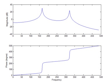
Figure 13. Bode diagram of 2 mass-spring-damper system.
In the models considered so far, mass is lumped into one point. A continuous structure such as a beam or string where the mass is distributed over volume requires another type of model. Figure 14 illustrates a beam structure pinned at both ends so that it can rotate but cannot translate. Under excitation, the beam will deform, vibrate and deform per different shapes depending on the frequency of the excitation as well as mounting method (boundary conditions) of the beam ends. The beam will have a first resonant frequency at which all its points will move in unison; at the first resonant frequency, the beam will take the shape shown to the right in Figure 14 labeled First Mode Shape. At a higher frequency, the beam will have a second resonant frequency and mode shape, and a third, and fourth, etc. Theoretically there are an infinite number of resonant frequencies and mode shapes.
However at higher frequencies, the structure acts like a low-pass filter and the vibration levels get smaller and smaller. The higher modes are harder to be excited and have relatively less effect on the overall vibration of the structure.
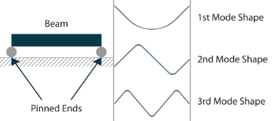
Figure 14. A beam fixed at both ends is an example of a continuous structure model.
Figure 15 shows an experimentally measured Bode Diagram for a 1 x 0.25 inch cross section and 8 inch long steel beam. There are many resonant frequencies, beginning as low as 265 Hz and many higher ones across the frequency range. Around every resonant peak, its phase goes through a 180 degree phase shift. Notice that when the resonances are well separated per frequency axis, the frequency response function of each resonance is similar to that of a simple spring-mass-damper system.
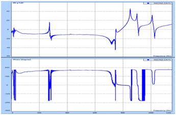
Figure 15 A typical Bode Diagram for a beam.
This overview of structural vibration analysis shows that the field has many complexities and considerable depth. Fortunately for technical and non-technical people alike, the fundamental phenomena and concepts apply to models no matter it is simple or complex, and they can be represented by either single-degree-of-freedom model, multiple-degree-of-freedom model, or continuous structure model.
Vibration Measurements
Vibration Sensors
Structural vibration is commonly measured with electronic sensors called accelerometers. These sensors convert an acceleration signal to an electronic voltage signal that can then be measured, analyzed and recorded with electronic hardware. There are many types of accelerometers. Some common one requires a power supply connected by a cable to the accelerometer as shown in Figure 16. Some accelerometers have internal circuitry that accepts the DC power from the analyzer's ADC channel. The dynamic signal analyzer includes a calibration setting parameter for each transducer that allows the voltage signal to be converted into the measurement of acceleration, i.e., g or m/s2.
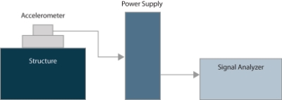
Figure 16. Typical instrumentation for accelerometer.
Manufacturers calibrate each accelerometer and supply a sensitivity value. For example, a 100 mV/g nominal sensitivity accelerometer will have a calibration value of 102.3 mV/g. Measurement accuracies depend on using the correct sensitivity value in the signal analyzer and on using an accelerometer with the right range of sensitivity for the application. A high sensitivity sensor with 1000 mV/g sensitivity may not be appropriate for an application of high acceleration level. In this case the too high voltage from the sensor will saturate the input channel circuitry on the signal analyzer. If the acceleration level is very low, a small sensitivity accelerometer, such as 10 mV/g one, may produce a signal that is too weak to measure and affect the accuracy of measurement.
Sensitivity also has an important impact on the signal to noise ratio. Signal to noise ratio is the ratio of the signal level divided by the noise floor level and typically measured in dB scale as:

All sensors and measurement hardware are subject to electronic noise. Even when the structure is not vibrate, electronic noise from the measurement elements may still shows some small acceleration level. This is due to the sensor cables picking up electronic noise from stray signals in the air, from noise in the power supply or from internal noise in the analyzer electronics. High quality hardware is designed to minimize the internal noise making low signal measurements possible. The signal to noise ratio limits the lowest measurement that can be made.
For example, if the noise floor is 1 mV, then with a typical 100 mV/g accelerometer, the smallest level that can be read, can be computed as:
1 mV divided by 100mV⁄g = 0.01 g
If a 20 g acceleration is measured with this accelerometer, then the signal to noise ratio can be computed as:

In this case, the analyzer will always show a level of at least 0.01 g because of the noise floor. It is a good practice to not trust a measurement with a signal to noise ratio that is below 3:1 or 4:1. When the signal to noise ratio is too low, one solution is to use an accelerometer with a higher sensitivity.
For example, with 1 mV of noise, the smallest level that can be read by a 1000 mV/g accelerometer can be computed as:
1 mV divided by 1000mV⁄g = 0.001 g
Some accelerometer power supplies include a gain setting that multiplies the signal by 1, 10, or 100. Unfortunately, this gain setting also amplifies the noise that is picked up by the wires and inherent in the sensor and power supply. In most cases, increasing the power supply gain will not solve signal to noise issues.
Section 3
Excitation MethodsIn some applications, vibration measurements are made during normal operation of a structure or machine. For example, an automobile can be instrumented with many accelerometers and driven on road or a test track while vibration signals are measured and analyzed. Many other cases require a more tuned excitation to yield reproducible and predictable results. The two most common methods are the impact hammer and electrodynamic shaker.
An impact hammer, as shown in Figure 17, is a specialized measurement tool that produces short duration vibration levels by striking the structure at certain point. The hammer incorporates a sensor (called a force sensor) that produces a voltage signal proportional to the force of impact. This enables precise measurement of the excitation force. An impact hammer is often used for modal analysis of structures where use of a shaker is not convenient; examples are in the field or with very large structures. Different impact tip materials allow tailoring of the frequency content of the impact force. For low frequency measurements, a soft rubber tip concentrates the excitation energy in a low narrow frequency range. A hard metal tip gives good excitation energy content out to high frequencies.

Figure 17. Impact hammer instrumented with a force sensor to measure the excitation force and different hardness tips
For laboratory vibration measurements, modal shakers are the instruments of choice. Modal shakers are rated by the force they produce. Modal Shakers vary in size and force from several pound force to hundred pound force.
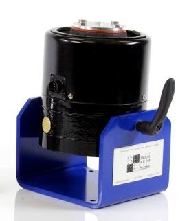
Figure 18. Modal shakers are used in laboratory measurements and vary in size from small to large.
Modal Shaker is connected to structures by means of a thin metal rod called a stinger in general. Force sensor is mounted on the structure, and then connected through the stinger to the modal shaker. There is a type of sensor called impedance head, which is a combination of force sensor and accelerometer in one. Using this sensor, both the driving force and acceleration level at the driving point on the structure can be measured simultaneously.
A dynamic signal analyzer incorporates a source type of signal, which is amplified and sent to the modal shaker to excite the structure under test.
Dynamic Signal Analyzers
The most common equipment for analyzing vibration signals is a computer based data acquisition system called a dynamic signal analyzer (DSA) (see Figure 19). The first generation DSAs used analog tracking filters to measure frequency response. Modern analyzers use digital technology and are far faster and more versatile. Using disk drives to store large volumes of data for post processing, they can record all sorts of data including time, frequency, amplitude and statistic data.
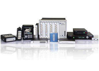
Figure 19. Crystal Instruments Dynamic Signal Analyzer family
A modern DSA consists of many electronic modules as shown in Figure 20. First, the analyzer measures electronic signals with an analog front end that may include special signal conditioning such as sensor power supply, TEDS (transducer electronic data sheets that read the calibration and other information from a chip embedded in the sensor), adjustable voltage gains settings and analog filters. Next, the system converts the analog signal to a digital format via an analog to digital converter (ADC). After the signal is digitized, the system processes it with a digital signal processor (DSP), which is a mini-computer optimized to do rapid mathematical calculations. The DSP performs all required calculations, including additional filtering, computation of time and frequency measurements, and management of multiple channel signal measurements.
Most modern signal analyzers connect with a PC for the setup, display ad reporting functions. The DSP interfaces with the PC; a software user interface displays results on the PC screen. Some older model of analyzers did not have a PC interface; they include buttons and a display screen on the analyzer chassis. The PC interface speeds and simplifies test setup and reporting.

Figure 20. Signal analyzer architecture
Quantization: Analog to Digital Conversion and Effective Bits
One measure of DSA quality is the bit count of the analog to digital conversion (Demler, 1991). When an analog signal is converted into a digital signal, it undergoes quantization, which means that a perfectly smooth analog signal is converted into a signal represented by stair steps as shown in Figure 21. To accurately represent an analog signal, the stair steps of the digital signal should be as small as possible. The step size depends on the number of "bits" in the ADC and the voltage range of the analog input. For example, if the voltage range is 10 volts and the ADC uses 16 bits, the smallest step size can be computed as,
Step size = 10 volts divided by 216 = 0.15 millivolts
A 24-bit ADC, reduces the step size to
Step size = 10 volts divided by 224 = 0.0006 millivolts
The 24-bit ADC has a step size that is 256 times smaller than the step size of the 16-bit ADC. Twenty four bit is the highest bit count available in modern DSAs. A 24-bit ADC can accurately measure large signals and small signals at the same time. ADCs with lower bit counts require the user to change to lower voltage range when measuring a low level signal in order to achieve the similar measurement accuracy.

Figure 21. When an analog signal is converted to digital the smooth analog signal becomes a stair step signal with the size of the step depending on the bit count of the ADC.
The bit count is also related to dynamic range of the DSA, another important measurement quality consideration. Dynamic range shows the ratio of the largest signal to the smallest signal that a DSA can accurately measure; dynamic range is reported in the dB scale. A typical 24-bit ADC with good low-noise performance will have 110 - 120 dB of dynamic range. Dynamic range is also affected by the noise floor of the device.
Measurement Types: time vs. frequency, FFT, PSD, FRF, Coherence
Most analyzers carries out time and frequency measurements. Time measurements include capturing transient signals, streaming long duration events to the computer disk drive, and statistic measures. The sampling rate, another measure of DSA quality, is related to time measurements. High speed ADCs can attain sampling rates of up to 100,000 samples per second (100 kHz). Some analyzers incorporate multiplexers that use one ADC sampling at a high rate and switch it between the different input channels. For example, if the DSA has 8 channels and a multiplexing 100 kHz ADC, it will only sample at 12.5 kHz per channel. High-quality DSAs do not use multiplexers and provide high sampling rates regardless of the number of input channels.
Most DSAs can compute a variety of frequency measurements including Fast Fourier Transform, Power Spectral Density, Frequency Response Functions, Coherence and many more. The DSP computes these signals from digitized time data. Time data is digitized and sampled into the DSP block by block. A block is a fixed number of data points in the digital time record. Most frequency functions are computed from one block of data at a time.
Fast Fourier Transform (FFT) is the discrete Fourier Transform of a block of time signal. It represents the frequency spectrum of the time signal. It is a complex signal meaning that it has both magnitude and phase information and is normally displayed in a Bode Diagram. Figure 22 shows the FFT of a square wave measured by a Crystal Instruments DSA Analyzer. The horizontal axis shows frequency ranging from zero to 225 Hz; the vertical axis is m/s2 ranging from 0 to 14 m/s2. A square wave is composed of many pure sine waves indicated by the discrete peaks at even intervals in the FFT.

Figure 22. FFT of a square wave computed with Crystal Instruments DSA Analyzer.
Power Spectral Density (PSD) is computed from the FFT by multiplying the FFT by its complex conjugate. The result of this operation is a real signal with power units (squared values) known as power spectrum. The phase information is gone, leaving only the magnitude data. The final computation is the division of the resulting power spectrum by the frequency increment. This step normalizes the measurement to the FFT "filter bandwidth" and converts the power spectrum into a density function. The advantage over non-density representations of spectra is that the level will not change when the frequency resolution is modified. The units of an acceleration signal PSD are (m/s)2/Hz. PSD measurements are used to analyze "stationary" signals such as random noise. Figure 23 shows the PSD of a broadband vibration signal displayed in LogMag units.

Figure 23. Power Spectral Density of broad band random vibration
Frequency Response Function (FRF) is computed from two signals. It is sometimes called a "transfer function." The FRF describes the level of one signal relative to another signal. It is commonly used in modal analysis where the vibration response of the structure is measured relative to the force input of the impact hammer or shaker. FRF is a complex signal with both magnitude and phase information.
Coherence is related to the FRF and shows the degree of correlation of one signal with a second signal. Coherence varies from zero to one and is a function of frequency. In modal analysis, this function shows the quality of a measurement. A good impact produces a vibration response that is perfectly correlated with the impact, indicated by a coherence plot that is near one over the entire frequency range. If there is some other source of vibration, or noise, or the hammer is not exciting the entire frequency range, the coherence plot will drop below one in some regions.
Most DSAs can compute many other time and frequency based signals including cross power spectrum, auto and cross correlation, impulse response, histograms, octave analysis, and order tracks.
Triggering, Averaging & Windowing
Getting good measurements from an analyzer requires careful selection of the measurement settings for the averaging, triggering, and windowing parameters.
Triggering is a technique for capturing an event when you do not know exactly when it will occur. A trigger can start data acquisition and processing when a user-specified voltage level is detected in an input channel. For example, you can set up a trigger to capture a hammer impact. After arm the trigger, the analyzer will wait until the impact occurs before it starts acquiring data.
Averaging improves the quality of the measurement. It applies to both the frequency and time domains. Frequency domain averaging uses multiple data blocks to "smooth" the measurements. You can average signals with a linear average where all data blocks have the same weight; or you can use exponential weighting. In this case, the last data block has the most weight and the first has the least. Averaging acts to improve the estimate of the mean value at each frequency point; it reduces the variance in the measurement. Time domain averaging is useful in measuring repetitive signals to suppress background noise. An impact test is good example of repetitive signals. Both the force and acceleration signals are the same for each measurement. This assumes that the trigger point is reliable. The presence of high background noise may adversely affect the reliability of the trigger.
Windowing is a processing technique used when computing FFTs. Theoretically, the FFT can only be computed if the input signal is periodic in each data block (it repeats over and over again and is identical every time). When the FFT of a non-periodic signal is computed, the FFT suffers from 'leakage.' Leakage is the effect of the signal energy smearing out over a wide frequency range. If the signal were periodic, it would be in a narrow frequency range. Since most signals are not periodic in the data block time period, windowing is applied to force them to be periodic. A windowing function should be exactly zero at the beginning and end of the data block and have some special shape in between. This function is then multiplied with the time data block, and this forces the signal to be periodic.
Figure 24 shows the effect of applying a Hanning window to a pure sine tone. The left top graph is a sine tone that is perfectly periodic in the time window. The FFT (left-bottom) shows no leakage; it is narrow and has a peak magnitude of one, which represents the magnitude of the sine wave. The middle-top plot shows a sine tone that is not periodic in the time window. This results in leakage in the FFT (middle-bottom). Applying the Hanning window (top-right), reduces the leakage in the FFT (bottom-right).
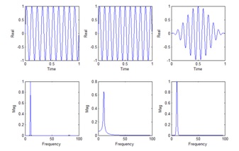
Figure 24. Hanning window (right) reduces the effect of leakage (middle)
FFT Settings: dF, dT, time window, span
Other important settings on the DSA include time and frequency resolution, and time and frequency span. A data block consists of some fixed number of data points that represent the digitized time record. The time between the points is called the time resolution, or dT. The time span of the data block can be computed from dT multiplied by the number of points. These parameters are set on the DSA and they affect the measurement results. If an event lasts a long time, you must set the system for a long time span. If the vibration levels change rapidly, use a smaller dT to capture the details of the time history.
There are two main parameters in the frequency domain: the frequency resolution, dF; and the frequency span. All frequency measurements are plotted with frequency on the horizontal axis. The dF defines the spacing between two points on the frequency axis. The frequency span defines the range between zero and the highest value on the frequency axis. These parameters are also set in the DSA. If the PSD shape changes dramatically over a short frequency range, use a small dF.
These four parameters cannot be selected independently because of the interrelations between them. The below equations summarize the relationships.
Frequency Resolution
dF (Hz) = 1/Time Period (sec)
0.5 second Time Period: dF = 1/0.5 = 2 Hz
Number of Frequency Points
Number Frequency Points = ½ Number Time Points
2048 time points yields 1024 frequency lines
Example:
Time Record: 2048 points, dT=0.001 sec, T= 2.048 sec
FFT: 1024 frequency lines, 0.488 Hz - 500 Hz
Displays: scaling, waterfall, spectrograph
In addition to two-dimensional plots, common display formats include orbit plots, waterfall plots and spectrographs. An orbit plot shows one time trace on the x axis and a second time trace on the y axis. A waterfall is a three dimensional plot made by stacking up consecutive two-dimensional plots. Waterfall plots show how a signal changes over time, or how a signal measured from a rotating machine changes with variations in the RPM. They are also useful for Order Analysis. Figure 25 shows a typical waterfall plot of the spectrum of the vibration measured on a rotating machine during a run-up and coast down. Often the waterfall plot includes an option to display one slice, and record of the waterfall in separate panes.
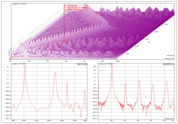
Figure 25. Time waterfall plot of PSD measured from a rotating machine during run-up with spectrum slice on top.
Waterfalls can also be presented as a spectrogram as shown in Figure 26, a two dimensional format using color to represent amplitude.

Figure 26. Spectrograph of rotating machine run-up shown in Figure 25.
Vibration Suppression
After taking vibration measurements and identifying problems, the next task is to fix them. This usually means suppressing by modifying the structure to eliminate the unwanted vibration effects. The many methods available for vibration suppression include source isolation, absorbers, damping treatment and active suppression. The examples that follow show techniques of vibration suppression in rotating equipment.
Isolation
Treating the source of the vibration is the most effective and often the most economical solution to vibration problems. The rotating unbalance in Figure 27 may cause the entire structure to vibrate. This can be solved by balancing the rotor and eliminating the vibration source. Another method of isolation is to add a highly damped material between the source and the structure. For example, on automobile engines large rubber mounts isolate the chassis from the engine.
Absorbers
When you cannot isolate the vibration source from the structure, another choice is to add a vibration absorber. The challenge is to absorb the vibration without affecting the structure. A vibration absorber is simply a mass-spring-damper system added to the structure and tuned to the same frequency as the offending vibration. An example is shown in Figure 27 where a vibration absorber is added to a rotating machine bracket to reduce the vibration of the bracket and surrounding structure. The mass-spring-damper system resonates and vibrates with large amplitudes, thus eliminating or reducing the vibration from the rest of the structure and reducing the vibration transmitted to other parts of the structure.

Figure 27. Vibration isolators (left) and absorbers (right) are methods of passive vibration suppression.
Damping Treatment
The most common form of vibration suppression is to add viscoelastic damping treatment to structural elements that are otherwise lightly damped. A thin steel beam may be highly resonant and exhibit large vibration that cause fatigue and failure, or transmit vibration to other parts of the structure. Applying an elastic coating to the steel surface increases the damping of the beam and thereby significantly reduces the vibration and its transmission. This method solves the problem with a negligible increase to the mass of the structure. Some structures use complex composite materials to increase the damping. The layered sheet metal used in automobile bodies is one example.
Critical Speeds of Rotating Equipment
Rotating machines such as turbines, compressors and shafts are particularly subject to imbalances that cause vibration. When the rotating speed corresponds to the resonance frequency of the first bending mode of the shaft, large forces are generated and transmitted to the bearings, eventually causing failure. This speed is called "critical speed," and the vibration is called "synchronous whirl." Rotating machines normally operate above the critical speed, so that the rotor must go through the critical speed to come up to full speed. If the run-up is too slow, the resonance at critical speed may build to unsafe levels. The rotor should have sufficient damping in the first mode to avoid this problem.
Active Vibration Suppression
When no other means of vibration suppression is feasible, active vibration suppression may be the only answer. Active suppression refers to using electronic controls to measure the vibration levels, process the data and drive a mechanical actuator to counteract the vibration levels as illustrated in Figure 28. It is analogous to the anti-noise sound suppression systems in airplanes and jets. Active suppression is expensive to implement and requires careful design that may be strongly dependent on the nature of the structure. Off-the-shelf active vibration suppression systems are not available.

Figure 28. Damping treatment is the most common and active suppression is the most expensive technique for vibration suppression.
Vibration suppression is a broad topic. It is best to start at the source and work down the transmission path when necessary. Most techniques add damping, or change the mass and stiffness to move the resonant frequencies away from fixed driving frequencies. However, changing the vibration response of one part of a structure is likely to change the vibration response of other parts as well.
Section 4
Modal AnalysisStructures vibrate in special shapes called mode shapes when excited at their resonant frequencies. Under normal operating conditions, the structure will vibrate in a complex combination of all the mode shapes. By understanding the mode shapes, all the possible types of vibration can be predicted. Modal Analysis refers to measuring and predicting the mode shapes and frequencies of a structure.
The mode shapes and resonant frequencies (the modal response) of a structure can be predicted using mathematical models known as Finite Element Models (FEM). These models use points that are connected by elements with the mathematical properties of the structure's materials. Boundary conditions define the method of fixing the structure to the ground and the force loads applied. After defining the model and boundary conditions, the FEM software computes the structure's mode shapes and resonant frequencies. This analytical model greatly aids in the design of a structure by predicting its vibration response before it is built. Figure 29 shows a Finite Element Model of a pressurized storage tank with force loads and boundary conditions.
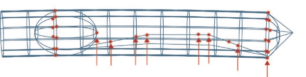
Figure 29. Finite Element Model of EADS Ariane 5 space vehicle.
After building the structure, good practice requires verifying the FEM using experimental modal analysis. This identifies errors, particularity in the assumptions on the boundary conditions, to help improve the model for future designs. Experimental modal analysis is also useful without FEM models because it can identify the modal response of an existing structure to help solve a vibration problem.
Experimental Modal Analysis consists of exciting the structure with an impact hammer or vibrator, measuring the frequency response functions between the excitation and many points on the structure, and then using software to visualize the mode shapes. Accelerometers measure the vibration levels at several points on the structure and a signal analyzer computes the FRFs (Frequency Response Functions).
Typically, the structure is divided into a grid pattern with enough points to cover the entire structure, or at least the areas of interest. The size of the grids depends of the accuracy needed. More grid points require more measurements and take more time.
One FRF measurement is made for every measurement location on the structure. The number of measurement points is determined by size and complexity of the structure and the highest resonant frequency of interest. High frequency resonances require a fine grid to fully determine the mode shape.
Each FRF identifies the resonant frequencies of the structure and the modal amplitudes of the measurement grid point associated with the FRF. The modal amplitude indicates the ratio of the vibration acceleration divided by the force input. The mode shape is extracted by examining the vibration amplitudes of all the grid points.
For example, the tuning fork shown in Figure 30 is a very simple structure that could reasonably be represented by a very few points. Say that three accelerometers are placed on points one through three and then impact hammer is used to excite the structure at point 4. A signal analyzer records the FRFs and produces the results shown in Figure 30. The resonant frequencies are the peaks that appear at every point at the same frequency. The amplitude of the peak at each location describes the mode shape for the associated resonant frequency.
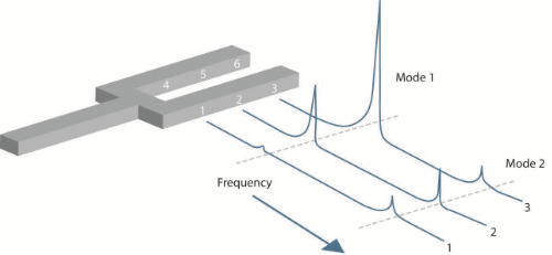
Figure 30. Modal analysis of a tuning fork results in FRFs for each point on the structure with the amplitudes at each resonant frequency describing the mode shape.
The results indicate that for the first mode, the base is fixed and the end has maximum displacement as shown in Figure 31. The second mode has maximum deflection at the middle of the fork as shown in Figure 31.

Figure 31. The first mode shape of the tuning fork has the base fixed and the maximum deflection at the end and the second mode shape has the ends fixed and maximum deflection at the middle.
Specialized software applications such as EDM Modal use FRF data to visualize the mode shapes. The software can identify the resonant frequencies and other modal parameters. Then it animates the mode shapes by drawing the deformed structure either with a static image or a moving animation showing deformation from one extreme to the other. The software can generate color plots such as the structure shown in Figure 32 to represent the amount of deformation.
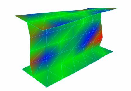
Figure 32. Modal analysis of an I-beam structure with deformed geometry and color shading.
The goal of modal analysis is to understand the mode shapes by visualizing the deformed geometry. This information helps to understand the structure deformation dynamically. For example, a consumer product may be failing in the field. It is suspected that vibration is the cause of this failure. It is also known that an internal cooling fan rotates at 3600 RPM, or 60 Hz. Modal analysis of the structure illustrates that the cooling fan mounting bracket has a resonant frequency with a bending mode at 62 Hz. This suggests that the fan is exciting the bending mode of the bracket and causing the failure. The bracket can be redesigned by stiffening its structure and increasing the resonant frequency to 75 Hz, thus avoiding the structural failure.
Operating Deflection Shape Analysis
Operating Deflection Shape Analysis (ODS) is similar to modal analysis. There are two types of ODS analysis: time-based and frequency-based. Time-based ODS collects the time records of the motion of points on the structure during normal operation. Then visualization software animates a geometric model of the structure so that moves in a manner proportional to the recorded data. Time-based ODS is different from modal analysis because there are no FRFs to record and no mathematical algorithms to apply.
It is analogous to videotaping the motion of the structure during normal operation and then playing it back to understand the motion. The advantage is that some measured motions may be too small to see with the naked eye. The software allows to increase the scale of these motions so that they can be visualized.
Frequency-based ODS animates the vibration of a structure at a specific frequency. Animated deformation shapes derive from frequency domain measurements such as auto-spectra or frequency response functions. Frequency-based ODS provides information on the relative levels of structural deformation. It is useful for cases where a force is applied and dwells at a specific frequency. It is a great tool for quickly spotting problems due to loose parts or connections. It is also useful for determining whether vibration will excite a resonance.
Conclusion
Structural vibration analysis is a multifaceted discipline that helps increase quality, reliability and cost efficiency in many industries. Analyzing and addressing structural vibration problems requires basic understanding of the concepts of vibration, the basic theoretical models, time and frequency domain analysis, measurement techniques and instrumentation, vibration suppression techniques, modal analysis, and more.
References
Demler, Michael J., "High-Speed Analog-To-Digital Conversion," Academic Press, Inc., San Diego, California 1991.
Hartmann, William M., "Signals, Sound, and Sensation," American Institute of Physics, New York, 1997.
Inman, Daniel J., "Engineering Vibrations, Second Edition," Prentice Hall, New Jersey, 2001.
Ramirez, Robert W., "The FFT, Fundamentals and Concepts," Prentice-Hall, New Jersey, 1985.
Ziemer, Rodger E., et. al., "Signals & Systems," Prentice Hall, New Jersey, 1998.