
Poly-X, the Poly-reference LSCF Implementation and Experiment
Abstract
A poly-reference least-square method for modal parameter identification of a system in frequency-domain is discussed and implemented. It can also be considered as a multi-reference frequency-domain implementation of the recognized time-domain based Least-Squares Complex Exponential (LSCE) estimator. The main advantages of the Poly-reference Least-Squares Complex Frequency-domain estimator (p-LSCF) are its capabilities of handling high system orders and high modal density. The stability diagram is much cleaner which makes the selection of system poles easier. Other advantages are lower computational times and the ability to handle multiple references. The Poly-X is Crystal Instruments’ version of p-LSCF, which is included in the EDM Modal software package. A MIMO FRF experimental test is carried out to demonstrate these advantages.
1. Introduction
Modal testing is usually performed to experimentally determine a dynamic system's modal characteristics. The results from modal tests are used to validate and improve FEA models, troubleshoot vibration and noise issues, and to study structural dynamics.
The rapid development of modal parameter estimation methods over the past few decades has not only increased the accuracy of modal parameter estimation but has also reduced the computational efforts. For modal parameter estimation, pole identification is the most critical part because poles contain useful information of vibration modes, such as natural frequencies and damping ratios. This report summarizes previous research on the least-square method for modal parameter identification in the frequency domain and focuses on pole identification. A test case is conducted to verify the implementation results of the p-LSCF method.
2. Implementation of Poly-X
Poly-X, the Poly-reference least-squares complex frequency-domain estimator (p-LSCF) is a poly-reference implementation of the LSCF estimator [1] and was first introduced in the [3]. One or more references can be handled by the p-LSCF method. When using one reference, the result is the same as the LSCF method. A simplified derivation is summarized here for implementation. Please refer to the original paper for a detailed derivation.
The relationship between the response (output) and excitation (input) in the frequency domain is modeled through the right matrix-fraction description (RMFD):

where Hˆ o(ω) is the model of measured FRF Ho(ω)∈CNf ×Ni
For output o = 1,2,...,No,

where  is the numerator polynomial of order n and

where D(ω)∈CNf ×Ni is the denominator polynomial of order n. The polynomial basis function Ωj (ω) is usually given by Ωj (ω)=(e-iω)j in the discrete-time domain. The βoj and Aj are coefficient matrix of polynomials which are the parameters to be estimated. Group these coefficients as θ = [βT1,…,βTNo,αT]T with

The coefficient matrix is estimated by minimizing the cost function:

By approximating the nonlinear least-square problem by a linear least-squares problem, the following cost function is obtained:

with

where

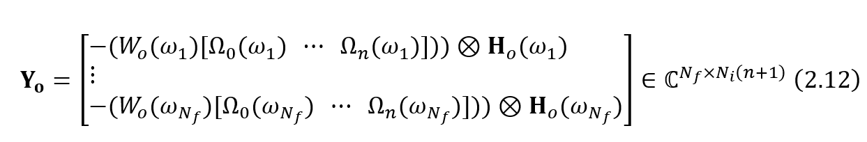
 represents Kronecker product and
 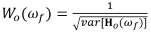 represents the weight applied on measured data.
To get the minimum cost function, both partial derivatives of Equation (2.7) with respect to β and α need to be zero.

Solve above two equations simultaneously:

Then calculate coefficient matrix α by solving least-square problem A⋅X = B from Equation (2.15):

The least-square solution of α is given by  , where INi is Ni×Ni identity matrix. The reason why use identity matrix to constrain highest order term of denominator polynomial was explained in [2]. Other methods for solving coefficient matrix and a detailed discussion on the effects of real and complex valued coefficient matrix can be found in [5]. Note that, on the demand of pole identification, only coefficients of denominator (α) are interested. Poles can be determined from eigenvalue problem as introduced in [4]:

where the eigenvalue matrix Λ contains the discrete-time poles z = e-sTs on its diagonal. Then transfer poles from z-domain to s-domain by s = -1/Tslnz. Natural frequency and damping ratio can be extracted by

Note: Poles with positive real parts are unstable poles, which can be eliminated before generating stability diagram.
3. Experimental Test Case

In order to compare the performance of Poly-X (p-LSCF) and typical time domain method (PTD), a modal shaker test is carried out on a rectangular (8” x 4”) plexiglass board (Figure 3.1). The plexiglass board is modeled with thirty-two 1” x 1” grids and has 45 measurement points in total. It is suspended from an elastic band which ensures a free-free boundary condition. The MIMO modal shaker test with roving response method is used in this experiment. One modal shaker with impedance head is mounted on No. 12 node and the other is mounted on No. 29 node to measure the -z (vertical) force. Three accelerometers are roved from node no.1 to no.45 during the experiment to measure +z response.
The MIMO FRF test enables both two modal shakers on nodes No. 12 and No. 29. Burst random signal (60% burst) of 0.05 V RMS amplitude was used as excitation signal. Frequency range of this test is set to 576 Hz, with a block size of 4096. No window is needed for burst random excitation method as the user can tune the burst percentage to control the no output duration time to ensure that the response decays naturally and there is no leakage.
With the help of a Mode Indicator Function (MIF), the natural frequencies can be labeled. By eliminating right body modes at extremely low frequencies and insignificant modes at high frequencies, modal modes were found between 50 and 350 Hz. A stability diagram generated based on PTD method is shown in Figure 3.3. A stability diagram generated based on Poly-X method is also shown in Figure 3.4. Comparison between the two estimation methods is discussed in the conclusion.

Figure 3.2: Measurement Tab displaying the test data

Figure 3.3: Stability diagram using PTD estimator

Figure 3.4: Stability diagram using Poly-X estimator
4. Conclusion
The Poly-X, a poly-reference least-square method is discussed and implemented. An experimental MIMO FRF test is carried out to exhibit its advantages. The Poly-X estimator produces a much cleaner stability diagram which simplifies the process of choosing the stable system poles. The poly-reference frequency-domain based estimator also works better in identifying lightly damped modes (Modes 1 and 2) and closely spaced modes (Modes 3 and 4) as observed in the stability diagrams procured from the different estimation methods. It was observed that using the same frequency band and same order of curve-fitting, the implemented Poly-X method is two times computationally faster than the PTD time domain estimator. These advantages make the Poly-X method more efficient and attractive.
[1] H. Van der Auweraer et al. “Application of a Fast-Stabilizing Frequency Domain Parameter Estimation Method”. In: Journal of Dynamic Systems, Measurement and Control 123 (2001), pp. 651–658.
[2] Bart Cauberghe et al. “The secret behind clear stabilization diagrams: the influence of the parameter constraint on the stability of the poles”. In: Proceedings of the 10th SEM international congress exposition on experimental and applied mechanics. 2004, pp. 7–10.
[3] Patrick Guillaume et al. “A poly-reference implementation of the least-squares complex frequency-domain estimator”. In: Proceedings of International Modal Analysis Conference. Vol. 21. 2003, pp. 183–192.
[4] Bart Peeters et al. “A new procedure for modal parameter estimation”. In: Sound and Vibration 38 (2004), pp. 24–29.
[5] Peter Verboven. “Frequency-domain system identification for modal analysis”. PhD thesis. 2004.