
Advanced Dynamic Signal Analysis
Download PDF | James Zhuge, Ph.D. - Chief Executive Officer | Simran Parmar - Applications Engineer | Prithvi Kanugovi - Applications Engineer
© Crystal Instruments 2023
Contents: 1. Introduction | 2. Swept Sine Measurements | 3. Acoustic Data Acquisition: Octave Analysis | 4. Acoustic Data Acquisition: Sound Level Meter | 5. Order Tracking | 6. Shock Response Spectrum Analysis | 7. Automated Test and Limit Check | 8. Real Time Digital Filters | 9. Histogram and Statistic Measures
1. Introduction
The CoCo and Spider hardware platforms can run in either DSA (Dynamic Signal Analyzer) or VCS (Vibration Control System) mode.
This DSA application note discusses the theory, EDM software and DSA operation for the optional advanced dynamic signal analysis features, including:
Swept Sine Analysis
Acoustic Data Acquisition: Octave Analysis and Sound Level Meter
Order Tracking
Shock Response Spectrum Analysis
Automated Test and Limit Test
Real Time Digital Filters
Histogram and Statistics Measures
Miscellaneous operations
Each topic includes a detailed description of the fundamental theory including mathematical formulation application topics, instructions to create a CSA file using the EDM software, and instructions to set up the data acquisition hardware to acquire measurements.
This document references the DSA Basics application note, which covers basic details of data acquisition hardware operations and basic frequency spectrum measurements including theory, EDM software set up, and DSA operations. Users are strongly recommended to read the DSA Basics application note prior to proceeding with this one.
This section describes the swept sine measurement capabilities of the DSA. It includes both theoretical background and application information. The Swept Sine Testing option has several unique advantages over similar products, including:
Measurement channels with a very high dynamic range ensure a continuous test over high dynamic range UUT (Unit Under Test). It is common to achieve 130~150 dB dynamic range using a CoCo-80 handheld signal analyzer.
Special tracking filters are realized based on TVDFT (Time Variant Discrete Fourier Transform) to provide excellent spectrum estimations.
Special algorithms enable tests in a wide frequency range. The results of both low and high frequency testing are excellent.
Time domain signals are always available for viewing and recording.
Log, Linear sweep modes are available.
Auto-gain adjustment with closed-loop control capability to prevent input range overloading.
Sine Signal Used for Testing
Broadband random, sine, step or transient signals are widely used as excitation signals in test and measurement applications. Figure 1 illustrates that an excitation signal x, can be applied to a UUT (Unit Under Test) and generate one or multiple responses denoted by y. The relationship between the input and output is known as the transfer function or frequency response function and represented by H(y,x). In general, a transfer function is a complex function that modifies the input signal magnitude and phase as the excitation frequency changes.

Figure 1. Left: a UUT with one response; Right: a UUT with two responses
With swept sine excitation, the characteristics of the UUT system can be measured experimentally. These characteristics include:
Frequency Response Function (FRF), which is described by:
Gain as a function of frequency
Phase as a function of frequency
Resonant frequencies
Damping factors
Total Harmonic Distortion.
Non-linearity
Others
Frequency response can be measured using the FFT cross power spectral method with broadband random excitation. Broadband excitation can be a true random noise signal with Gaussian distribution, or a pseudo-random signal of which the amplitude distribution can be defined by the user. The term “broadband” may be misleading, as a well implemented random excitation signal should be frequency band-limited and controlled by the upper limit of the analysis frequency range. That is, the excitation need not excite frequencies above that which can be measured by the instrument. The DSA random generator will only generate random signals up to the analysis frequency range. This will also concentrate the excitation energy on the useful frequency range.
The advantage of using broadband random excitation is that it can excite the whole frequency range in a short period of time, so the total testing time is less. The drawback of broadband excitation is that its frequency content is spread over a wide range within a short duration. The energy contribution of the excitation at each frequency point will be much less than the total signal energy (roughly, it is -30~ -50 dB less than the total). Even with many averaging in the FRF estimation, the broadband signal will not effectively measure the extreme dynamic characteristics of the UUT.
Swept sine measurements, on the other hand, can optimize the measurement at each frequency point. Since the excitation is a sine wave, all its energy is concentrated at a single frequency, eliminating the dynamic range penalty in a broadband excitation. In addition, if the frequency response magnitude drops, the tracking filter of the response can help to pick up extremely small sine signals. Simply optimizing the input range at each frequency can extend the dynamic range of the measurement to beyond 150 dB.
Introducing Sweeping Sine
A sine signal with a fixed frequency f0 can be expressed as:
x(t) = sin(2πf0t)
where t represents time. A sweeping sine signal has a changing frequency that is usually bound by two limits. The frequency change can be either in the linear scale or logarithmic scale based on different user requirements. The swept sine signal can be defined by the following parameters:
- The low frequency boundary, which is simply called Low Frequency or fLow
- The high frequency boundary, which is simply called High Frequency or fHigh
- The sweeping mode, either logarithmic or linear
- The sweeping speed, in either octave/min if the sweep mode is logarithmic, or in Hz/Sec if the sweeping mode is linear
- The amplitude of the sine signal, A(f, t), which can be a constant or a variable of time and frequency.
x(t)=A(f,t)*sin (2π(f(fLow,fHigh,Speed))t)
The instantaneous frequency f (fLow, fHigh, Speed) represents the current frequency of the sweeping sine. It is a changing variable and is usually displayed on the screen as Sweeping Frequency.
The sweeping frequency can also be manually controlled during the test with the Hold, Resume, Jump or Pause controls.
Unlike some DSA products that use swept sine tests with multiple discrete stepped sine tones in a sequence, the CI swept sine test uses a true digital synthesizing technique to generate sine sweeps with an extremely smooth analog-like transition from one frequency to another. This ensures that there are no sharp transitions during the test that might “shock” the UUT. The picture below shows a typical swept sine signal with 1.0 Vpk. (Figure 2)

Figure 2. Typical digitally synthesized swept sine signal
Sweeping Mode: Logarithmic or Linear
A swept sine can sweep in either linear or logarithmic mode. Linear sweep means the frequency will change at a constant speed, with units of Hz/sec. In this case the sweep rate is constant and the same at all frequencies.
Alternatively, the sweeping mode can be set as logarithmic or Log. In Log mode, the sweeping speed is slower at low frequencies and fast at higher frequencies. In Log mode, the sweeping speed units are in Octave/Min. 1.0 Oct/min which means that the frequency will take one minute to double from 1 kHz to 2 kHz, from 100 Hz to 200 Hz, or from 0.5 Hz to 1.0 Hz.
Most testing specifications request logarithmic sweeping for two reasons. The first is because it takes longer to measure one or multiple sine cycles at a low frequency versus a high frequency. The second is that most mechanical and electrical systems exhibit characteristics that are better described in a logarithmic frequency scale. This is because dynamics such as resonant frequencies occur over large frequencies spans: some at low frequencies and some at high frequencies. If linear sweeping is adopted, the user may find that whatever speed is chosen, it is either too slow in the high frequency end or too fast in the low end. Log sweeping mode solves this problem.
Once the sweeping mode is set to either Linear or Log in a DSA test, the frequency distribution of the display signals will be set to linear or logarithmic accordingly. This is discussed in the following section about the display resolution. The sweeping speed unit will automatically be set to Hz/Sec or Oct/Min.
Resolution of Display Signals
The sweeping sine signal is point-by-point digitally synthesized in the DSA. It has “infinitely” fine resolution in the frequency transition. It does not jump from one frequency to another.
The sweeping signal is displayed after the size of the displaying signals are set. (e.g.,1024 or 2048.) The DSA will distribute the frequency bins between fLow, fHigh. In Linear mode, the frequency spacing between two adjacent lines is represented by the frequency resolution; In Log mode, the frequency spacing between two adjacent lines of the signal will be represented by a ratio.
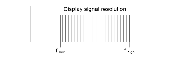
Figure 3. Spectrum resolution
For example, if a linear sweep is defined with flow = 100 Hz; fhigh = 1000 Hz, Signal Size = 1024, then the first line of the signal will be allocated to 100 Hz, the last to 1000 Hz. The frequency bins of the signals will be evenly distributed with frequency resolution of:
(1000-100) / (1024-1) = 0.879765 Hz
If a logarithmic sweep is defined with Log Sweep Mode: fLow = 100 Hz; fHigh = 1000 Hz, Signal Size = 1024, then the first line of the signal will be allocated to 100 Hz, the last to 1000 Hz. The Frequency resolution will be represented by a ratio as:
1000 Hz = 100 Hz * ratio(1024 - 1)
ratio = (1000/100)1/1024-1 = 1.00225335
This means that if the first line is at frequency 100 Hz, the second line will be at 100.225335 Hz, the third at 102.0045 Hz and the1024th line at 1000 Hz.
Once allocated, the display signals will keep the history of each calculated result. The DSA will update the points that are near the instantaneous frequency of the sweep. This is how the display signals are created. This design allows users to understand that increasing the resolution of the display signals will not increase or decrease the quality of the swept sine.
Tracking Filters
Historically, swept sine tests were originally conducted using analog technology where sine generation and measurements were all implemented in the analog domain. A very simple swept sine testing instrument consists of the following components:
A sine oscillator of which the frequency can be changed.
An RMS estimator to the output source.
An RMS estimator to the input signal.
A divider that divides the RMS measurements between input and output.
A display or plotter to show the divided results.
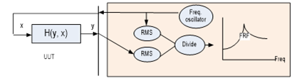
Figure 4. Analog swept sine implementation
The UUT response is not linear in many cases. The response signal may contain strong harmonics with very pure sine excitation. For example, with a sine tone excited at 100 Hz, the response signal may contain a response at 200 Hz, 300 Hz and so forth. A simple RMS estimator will not be able to distinguish the amplitudes at these additional responses, and as a result the FRF calculation will not be accurate.
To overcome this problem, users can apply a tracking filter that centers at the sweeping frequency and apply an RMS estimator to the output of the tracking filter as shown in Figure 5.

Figure 5. Tracking filter implementation
With a filter in place, the RMS estimator will accurately measure the frequency amplitude at the sweeping frequency. The energy at other frequencies will be filtered out.
The challenge of realizing such a filter in the swept sine test is that the filter has to track the center frequency of the sine frequency. Not only does the center frequency of the filter need to change, but also the bandwidth. To give an example, when the sweeping frequency is at 100 Hz, it is reasonable to use a filter bandwidth of 50~100 Hz. When the sweeping frequency goes down to 10 Hz, the next harmonics will be at 20 Hz. A filter with a bandwidth of 50~100 Hz will be too wide to use. To address the problem, a so called tracking filter is used. The tracking filter will change both the center frequency and bandwidth according to the sweeping frequency. Analog manufactured swept sine equipment would realize this by mixing frequency technology with expensive electronic components. Digital technology now allows users to implement digitally synthesized tracking filters in the software at no additional hardware cost.
The bandwidth of the tracking filter is a key control parameter. In DSA, it is defined as a percentage of the sweeping frequency. The user can select a percentage between 100% and 7%. A percentage of 100% means the equivalent bandwidth of the tracking filter is the same as its sweeping frequency. 50% means its bandwidth is ½ of the sweeping frequency.
Crystal Instruments DSA uses a proprietary digital filter that provides a very fast response and clean detection of the sine RMS value.
Measurement Quantities
Measurement quantities that can be monitored during the swept sine test include the time stream of each channel (raw data), spectrum of each channel, frequency responses, coherence, and phase between responses to the reference channel.
Time streams: time streams appear the same as any other applications on DSA. Time streams are always available for viewing and recording. This tool is very useful for observing whether the input signals are in the valid range. The recorded sine wave can be used for further post-processing.
Spectra: The term spectrum is used to refer to the measurement trace in the frequency domain of each channel. It is represented in 0~Peak. The engineering unit of the spectrum is determined by the sensor used by the input channel. The resolution of spectra does not affect the quality of sine wave.
Frequency Response Functions (FRF): FRF of UUT can be measured by taking a ratio of the response and excitation of the UUT.
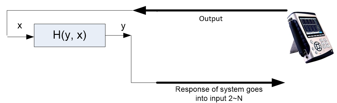
Figure 6. Frequency response measurement with CoCo
The DSA will provide the FRF functions of each response channel to the output channel. FRF signals include both phase and magnitude information. In DSA, the FRF is often denoted as Hyx.
The number of FRF signals that can be monitored depends on the number of input channels on the DSA hardware. For example, a CoCo-80 with 4 input channels can measure 3 FRFs: H(ch2,ch1), H(ch3,ch1) and H(ch4,ch1).
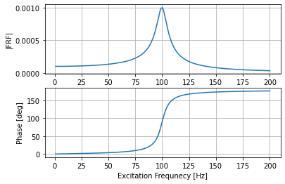
Figure 7. Frequency response function
When measuring the ratio between two response channels, it is more accurate to refer to the signals as Transmissibility functions instead of FRF because the reference signal is not really the excitation to the UUT. Figure 8 shows how to connect and measure the transmissibility between two response channels.
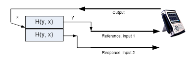
Figure 8. Typical transmissibility measurement
Transmissibility measurements are used in many applications. For example, it can be used in a “back-to-back” transducer calibration where an accurate reference transducer is used to calibrate a less accurate one.
Output Control Modes
Recall that the sine tone amplitude can be a variable of time and frequency.
x(t) = A(f,t)*sin (2π(f(fLow,fHigh,Speed))t)
We have discussed how the frequency can be changed and controlled by the sweeping mode, sweeping range, and sweeping speed. This section discusses how the output amplitude A(t) is controlled.
There are three Output Modes provided in a typical DSA:
Constant Output Level
Output Level Profile
Input Profile with Auto Gain Control
Constant Output Level
A(f,t) = constant
The Constant Output Level is the simplest way to generate the output. It uses a constant output level that is usually defined in the 0~peak volt. For example, a 1 Vpk means the output swept sine is in 1 V in 0~peak.
When the constant output level is used, the response may show peaks or valleys.
Figure 9 shows that a constant level sweep is applied to a Single Degree of Freedom (SDOF) device. The voltage output of the DSA will be converted to force using a mechanical excitation system. We would expect the response measured in either displacement, velocity or acceleration will show a resonant peak.

Figure 9. Constant output level
The drawback of using constant level mode is that sometimes the dynamics of the system vary to extremes such that the response signal may exceed the input range. This is very common with systems that have light damping. For example, a UUT with 60 dB dynamic range, which is quite common, will show the magnitude of the response change 1000 times over the test.
Output Level Profile
The output level A(f,t)=A(f) is defined by the user. It is possible to attenuate the excitation signal at certain frequency ranges to overcome problems with large variation of responses. In the example above, because the resonance frequency is likely known to the operator, we can set the output to a lower level in that specific sweeping frequency range. This frequency dependent output level control is referred to as the Output Level Profile. (Figure 10)

Figure 10. Output level profile
Figure 10 shows that we purposely created a notch in the output level profile so that the response signal is attenuated in the resonance area.
Modifying the output to a frequency dependent signal can improve the FRF or transmissibility measurement. It is much better than a constant level output. The drawback of this method is that the UUT dynamics must be known before the test. Another issue is that the output level profile may not be created accurately to match the dynamic characteristics of the UUT. To overcome this difficulty, the DSA also includes a close-loop control method to allow auto-gain control.
Auto Gain Control
Auto gain control calculates A(f,t) in real time based on the target input and close-loop control gain. This advanced method is explained in Figure 11.
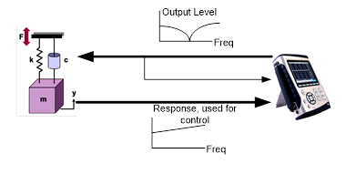
Figure 11. Auto gain control mode
First the user must set up the target profile for one of the response channels (input to the DSA). The shape of this target profile (Input Profile) does not need to be a straight line. Then during the sweep, the DSA measures the transfer function between the response and the output. Taking this transfer function into consideration, the DSA automatically adjusts its output so that the magnitude of the measured input signal matches the input control profile. As the transfer function changes with frequency, this method requires a close-loop control logarithm.
The input profile with auto-gain control is the most effective way to excite the system. It can maximize the dynamic range of the input channels. However, care must be taken so that the output channel does not get too large and the input channel is saturated, or the output channel gets too small and the input channel reduces to the background noise level.
Note that the Output and Input Profiles have different engineering units. The Output Profile always has the engineering unit of V [pk] for a sine wave. The Input Profile will have the engineering unit of whatever is measured by that channel. For example, if the response sensor is a displacement sensor, then the Input Profile will have displacement units, in 0~Peak. If it is an accelerometer, then it will have acceleration units, in 0~Peak.
When the Input Control Profile is selected, channel 2 is used as the control channel by default. You can select any channel other than the reference channel (channel 1) for control.
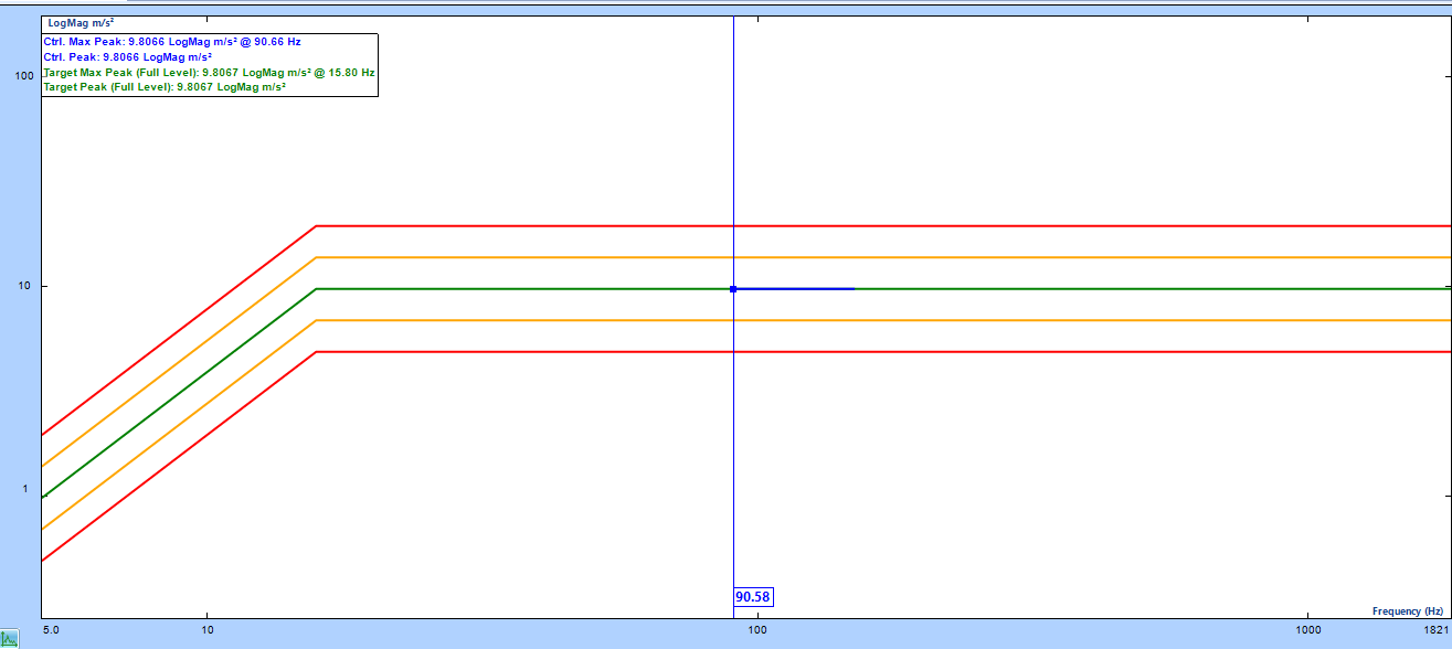
Figure 12. Input auto gain control mode profile
Sweeping Range and Profile
The sweeping range is controlled by the two boundaries of the frequency range. If the profile setting is not at the same range of the sweeping range, then the DSA will automatically adjust the range.

Figure 13. Sweeping range and profile
In Figure 13, the thick line represents the profile. If the Low Freq or High Freq limits do not match the Profile, the software extends the left and right ends to always find valid profile value points when the output sweeps.
Sweep Control
The swept sine output is controlled by sweeps. One sweep indicates that the output will generate the sine frequency from the Low Frequency to the High Frequency, or high to low. In addition, users can control the sweep with manual controls that include the following:
Start Output: start output the sine wave
Stop Output: this action will abort the test
Reverse Direction
Jump to Frequency
Hold Sweep: this action will not ramp down the output voltage amplitude. The frequency will be fixed.
Resume Sweep
Clear Display History

Figure 14. Sweep control options
To avoid shocking the UUT, a sine output will never start or stop abruptly. Instead, the sine wave amplitude slowly ramps up from zero to the desired level. The ramping rate is defined as dB/sec. 40 dB/sec means the sine wave will ramp up or ramp down by 100 times in magnitude per second. This is a user-defined advanced value.
The Acoustics Data Acquisition software option includes Fractional Octave Filter Analysis, Sound Level Meters. Microphone Calibration function is included.
The Fractional Octave Filter Analysis applies a bank of real-time octave filters to the input time streams and generates two types of signals at the same time: fractional frequency band signals, i.e., octave spectra and the RMS time history of each filter band. The output of each real-time filter bank is in fact a 3D waterfall signal that is arranged in the x-axis as logarithmic frequency and z-axis as time. In the frequency direction, frequency weighting is applied. In the time axis, the time-weighting is applied.
The Sound Level Meter (SLM) is a similar application to octave filters in acoustic data acquisition. This application is also referred to as an Overall Level Meter. The SLM applies ONE frequency weighting filter to the input signal and time weighting to the output. Various measures are then extracted from both the input and output signals of this frequency weighting filter.
Fractional Octave Filter Analysis
Acoustics Analysis provides 1/N octave analysis using true real-time digital filters that conform to ANSI std. S1.11:2004, Order 3 Type 1-D and IEC 61260-1995 specifications. A, B and C weighting filters can be applied to the input data. Output results are weighted or un-weighted RMS values. The output can be normalized with a calibration value. The results can be plotted on log or linear axes and exact or preferred frequency values are supported.
Each band filter is designed in accordance with ANSI S1.11 and IEC 61260 specifications by transforming the original analog transfer function to the digital domain by means of the bilinear transform. The filter order can be specified, and the frequency ratio can be calculated using the binary or decimal system.
The RMS reading of each octave filter is usually represented by a “bar” in the spectrum plot. Keep in mind that the octave filters have “skirts” on both sides. They are not as straight as the bars depicts. The adjacent filters always overlap. Due to this reason, a sine tone at 1 kHz will not only excite the filter with center frequency at 1 kHz, but also all other filter bands. Figure 15 shows how the energy in each band is displayed on the octave spectrum plot using bars.

Figure 15. 1/3 octave filter banks
Full Octave Filters
An octave is a doubling of frequency. For example, frequencies of 250 Hz and 500 Hz are one octave apart, as are frequencies of 1 kHz and 2 kHz.

Figure 16. Full octave filter shape
Full octave analysis, i.e., 1/1 octave, displays the frequency characteristics of a signal by passing the signal through a bank of band-pass filters where the center frequency of each filter is one octave apart. If the lower and upper cutoff frequencies of a band-pass filter are fL and fH, then the center frequency, fc can be determined with:
fc = √(fL * fH)
The nominal frequency ratio G is determined by:
G = fH/(fL
Base-two or base-ten systems are used in industry. G = 2 for base-two systems and G = 103/10 for base-ten systems. The Crystal Instruments DSA uses a base-ten system.
The proportional bandwidth property will divide the frequency information uniformly over a log scale. This feature is very useful for analyzing a variety of natural systems. For example, the human response to noise and vibration is very non-linear and many mechanical systems have a behavior that is best characterized by a proportional bandwidth analysis.
Fractional Octave Filters
To gain finer frequency resolution, the frequency range can be divided into proportional bandwidths that are a fraction of an octave. For example, with 1/3 octave analysis, there are 3 band-pass filters per octave where each center frequency is 101/10 the previous center frequency.
In general, for 1/N octave analysis, there are N band pass filters per octave such that:
fH/fL = (103/10)1/N
fc j+1 = fc j * (103/10)1/N
where 1/N is called the fractional bandwidth resolution.
For DSA, the equation and table below define the center frequency of each fractional filter.
fc = 103X/10N
For example, for 1/1 Octave (N =1) the first center frequency (index X = -3) is computed as
fc = 103*(-3)/(10*1) = 0.125 Hz
| 1/1-Octave | 1/3-Octave | 1/6-Octave | 1/12-Octave | |
|---|---|---|---|---|
| Standard | IEC 225-1966 DIN 45651 ANSI S1.11-2004 Order 7 Type 1-D |
IEC 225-1966 DIN 45651 ANSI S1.11-2004 Order 3 Type 1-D |
N/A | N/A |
| X (index) | -3 ~ 14 | -10 ~ 43 | -20 ~ 86 | -40 ~ 172 |
| Total number of filters | 18 | 54 | 107 | 213 |
| fc (Hz) | 0.125 – 16k | 0.1 – 20k | 0.1 – 20k | 0.1 – 20k |
Table 1: Octave Center Frequencies
Nominal Center Frequencies (midband frequencies)
Nominal center frequencies are “round” numbers that were inherited from the old analog octave filters. They are rounded midband frequencies for the designation of band pass filters. The nominal midband frequencies for 1/1-octave and 1/3-octave are listed in the ANSI S1.11-2004 Annex A. The standard also describes how to decide the nominal midband frequencies for other fractional octave bands.
The exact center frequency of the filter band is usually not identical to the nominal frequency. For example, in a 1/3 octave, the exact center frequencies of 794.33 Hz, 1000 Hz and 1258.9 Hz are used to correspond to filters with nominal frequencies of 800 Hz, 1000 Hz and 1250 Hz.
Band Edge Frequencies of Fractional Filters
The low and high edge frequencies of a filter can be calculated based on the frequency ratio, G (103/10) and the fractional octave resolution N (=1, 3, 6, 12…),
Lower edge frequency,
fL = fc * (103/10)-1/2N
Upper edge frequency,
fH = fc * (103/10)1/2N
The bandwidth of the filter is:
BW = fc - fL
When starting or resetting the filtering operation of the fractional-octave filters, a certain time is required before the measurements are valid. This time is called the settling time and is related to the bandwidth of any filter. The lowest frequency band has the smallest bandwidth and defines the settling time required before the user can consider the complete fractional-octave measurement valid. A good rule of thumb is that the settling time is approximately five divided by the bandwidth.
Settling time = 5/BW = 5/(fc - fL)
Note the settling time depends on the bandwidth which changes with the center frequency. A narrower filter and a lower frequency band requires a longer settling time.
Analysis Frequency Range
In DSA, the user can decide the analysis range by changing the lowest and highest fc as the Analysis Parameters in Table 2.
| Analysis Range | 1/1 Octave | 1/3 Octave | 1/6 Octave | 1/12 Octave |
|---|---|---|---|---|
| Lowest fc (Hz) | 0.125 1 8 |
0.1 1 10 100 |
0.1 1 10 100 |
0.1 1 10 100 |
| Highest fc (Hz) | 1000 4000 16000 |
1000 2000 5000 10000 20000 |
1000 2000 5000 10000 20000 |
1000 2000 5000 10000 20000 |
Frequency Weighting
The human hearing system is more sensitive to some frequencies than others, and its frequency response varies with level. In general, low frequency and high frequency sounds appear to be less loud than mid-frequency sounds, and the effect is more pronounced at low pressure levels, with a flattening of response at high levels. Octave analysis and sound level meters therefore incorporate weighting filters, which reduce the contribution of low and high frequencies to produce a measurement that corresponds approximately to what we hear.
DSA provides A, C, Z weightings conforming to IEC 61672-1 2002 and B weighting conforming to IEC 60651 in both Octave Analysis and Sound Level Meter. The frequency weighting in the octave filters will affect the results of all filter bands.

Figure 17. Frequency weighting filter shapes
Time or RPM based RMS Trace of Octave Filters
The ANSI and IEC standard does not require the time history of the band pass filter output to be stored. Users can find the RMS history of all band pass filters are stored on the DSA in the RMS quantity. The following is a description of how the RMS history is calculated.
The RMS history can be stored against one of two variables: Time or RPM.
Both the input and output of a digital filter are a series of data points. While it requires excessive memory to keep all the time data of all the filters, it is useful to keep the so-called RMS history of each filter output. The RMS time history is computed after the time weighting averaging operation as shown in Figure 18.

Figure 18. RMS time history calculation
The Decimator is used to allow the user to select a length of time to save the RMS data. For example, given a buffer length of 1024, a Trace Update Time of 5 ms will keep about 5 seconds of RMS history. If this update time is set to 5 seconds, it will record 1.4 hours of RMS history.
Figure 19 shows the 3D waterfall display of a 1/1 octave filter output. If a cut is made in the Z axis direction, the result will be an octave spectrum. If a cut is made in the X-axis, the result is called a Time Trace.
Figure 19. A cut of 3D Waterfall of octave filter output (top) maps to an RMS time trace (bottom)
The DSA allocates one Time Trace for each channel to display. Keep in mind that this buffer of Time Trace is the output of a specific filter, the user can change the center frequency of the filter for the Time Trace during run time. In other words, this time trace display buffer will change its content completely when the user switches the Time Trace Frequency from one to another.
Alternatively, the RMS trace can be stored using RPM as a variable. This method is particularly useful in the automotive NVH applications. The following figure illustrates how one of the filter outputs can be stored in a RPM trace.

Figure 20. Store RPM based RMS traces
Exponential and Linear Averaging
Linear average: The Linear average method uses a fixed time period to sum up the historical power value of each filter and then takes the square-root to calculate the averaged RMS value. In Linear average, the RMS trace update time is governed by the time period of averaging. One RMS value per frequency bin is produced for each time period of averaging.
Exponential average: Exponential average applies an exponential time constant to the historical power values of each filter and takes the square-root of the averaged power value. A time constant of 0.125 seconds is equivalent to “Fast” averaging and 1.0 second is equivalent to “Slow” averaging in the acoustics. In exponential average, the RMS trace update time is independent of the time constant.
Peak Hold: Peak Hold retains the maximum value in each frequency bin over the period of time since last “start” or “restart”.
As discussed previously, each filter may have a different settling time.
DSA Measurements in Octave Analysis Mode
The following measurement quantities are available on the DSA in octave measurement mode.
Time streams of input channels
In DSA, time domain data is always available in the form of long-time history. The user can view and record the time signals. The limitation is that the sampling rate of the time signals cannot be arbitrarily changed. It is always set internally by the system based on the analysis frequency range, i.e., the highest center frequency of the filter bands.
Octave Spectra
Each input channel will have an octave spectrum.
RMS Trace
Each input channel will have one RMS trace to display the RMS history. This RMS is the output of the filter for a specific band. The RMS trace is defined as the Time-RMS trace or RPM-RMS trace at the CSA Editor level. You cannot switch from Time to RPM based during a CSA.
An analog sound level meter measures the sound pressure level. The standard sound level meter is more accurately referred to as an exponentially averaging sound level meter since the AC signal from the microphone is converted to DC by a RMS circuit and thus requires a time-constant of integration. This is referred to as time-weighting. Three of these time-weightings have been standardized: 'S' (1 s) originally called Slow, 'F' (125 ms) originally called Fast, and 'I' (35 ms) originally called Impulse. The output of the RMS circuit is linear in voltage and is passed through a logarithmic circuit to give a readout in decibels (dB). This is 20 times the base 10 logarithm of the ratio of a given root-mean-square sound pressure to the reference sound pressure. Root-mean-square (RMS) sound pressure is obtained with a standard frequency weighting and standard time weighting.
The advent of digital technology and the increasing accuracy of electronic circuits has advanced sound level meter functions, which are more recently calculated in the digital domain. One of the important factors of this implementation is that the instrument must provide a very high dynamic range to allow both weak and strong signals to be calculated and observed. Crystal Instruments DSA provides up to 130 dB dynamic range. High dynamic range is one of the most important quality standards of an acoustic analyzer.
A traditional sound level meter only includes the 1/1 and 1/3 octave filters. In the DSA system, octave analysis is provided in addition to other analysis functions to facilitate more flexibility and computation power compared to a traditional sound level meter.
Octave Analysis provides templates for projects requiring fractional octave analysis. Frequency weighted readings (such as dBA) are available in both Octave Analysis and Sound Level Meter templates. Reading results may be slightly different when comparing Octave Analysis and Sound Level Meter results. This is because the data processing flow in octave filter analysis and sound level meter is computed differently. In the octave analysis, the dBA, i.e., the A-weighted sound level is computed by applying the frequency weighting function to the output of each individual filter bank, whereas in SLM, the A-weighted sound level is created by applying the A-weight filter to the entire time domain. The SLM template should be used to obtain the dBA or similar overall readings for sound studies that might compare results with a traditional sound level meter because the computation is similar.
Terms and Definitions
This section defines the terminology used in the SLM software options.
Reference sound pressure
It is conventionally chosen as 20 μPa. This is the threshold of hearing for the average person and is used to compute the sound pressure level in the dB scale.
Sound pressure level (in dB)
Sound pressure level (dB) is defined as twenty times the logarithm to the base ten of the ratio of the RMS of a given sound pressure to the reference sound pressure.
The sound pressure level is expressed in decibels (dB) and the symbol LP.
Peak sound pressure
The peak sound pressure is the greatest absolute instantaneous sound pressure during a stated time interval.
Peak sound level (in dB)
The peak sound level (dB) is defined as twenty times the logarithm to the base ten of the ration of a peak sound pressure to the reference sound pressure, peak sound pressure being obtained with a standard frequency weighting.
(Example letter symbols are Lpeak , LCpeak , LCpeak)
Frequency weighting
Frequency weighting is the difference between the level (dB) of the signal indicated on the display device and the corresponding level of a constant-amplitude steady-state sinusoidal input signal, specified in the IEC or ISO standards as a function of frequency. It accounts for A, B and Z frequency weightings as discussed in the previous section.
Time weighting
Time weighting is an exponential function of time of a specified time constant that weights the square of the instantaneous sound pressure. This is the same as exponential averaging in the time domain to the instantaneous sound pressure.
It is a continuous averaging process that applies to the output of a frequency weighting filter or one of the fractional filters. The amount of weight given to past data as compared to current data depends on the exponential time constant. In exponential averaging, the averaging process continues indefinitely.
In a sound level meter, the time weighting exponential averaging mode supports the following time constants:
Slow uses a time constant of 1,000 ms. Slow averaging is useful for tracking the sound pressure levels of signals with sound pressure levels that vary slowly.
Fast uses a time constant of 125 ms. Fast averaging is useful for tracking the sound pressure of signals with sound pressure levels that vary quickly.
Impulse uses a time constant of 35 ms if the signal is rising and 1,500 ms if the signal is falling. Impulse averaging is useful for tracking sudden increases in the sound pressure level and recording the increases to provide users with a record of changes.
User Defined allows the user to specify a suitable time constant for a particular application.
Time-weighted sound level (in dB)
This is twenty times the logarithm to the base ten of the ratio of a given RMS sound pressure to the reference sound pressure, RMS sound pressure being obtained with a standard frequency weighting and standard time weighting.
(example letter symbols are LAF, LAS, LCF, LCS)
Maximum and minimum time-weighted sound level (in dB)
This is the greatest and lowest time-weighted sound level within a stated time interval.
(example letter symbols are LAFmax, LASmax, LCFmax, LCSmax, LAFmin, LASmin, LCFmin, LCSmin)
Time-average sound level (equivalent continuous sound level) (in dB)
This is twenty times the logarithm to the base ten of the ratio of a RMS sound pressure during a stated time interval to the reference sound pressure, sound pressure being obtained with a standard frequency weighting. (example letter symbols are Laeq, Lceq))
Sound exposure
This is the time integral of the square of sound pressure over a stated time interval or event.
Sound exposure is used to measure high-level, short duration noises and to study their effects on humans.
Sound exposure level (in dB)
Sound exposure level is the total sound energy of a single sound event considering both its intensity and duration.
Sound exposure level is the sound level experienced if all the sound energy of a sound event occurred in one second.
This normalization to a duration of one second allows the direct comparison of sounds with different durations.
The Leq is the constant level needed to produce the same amount of energy as the actual varying sound (the SPL).
The SEL is the Leq normalized to 1 second. It is what the Leq would be if the event occurred over a one second duration.
Statistical level (LN)
LN is defined as the sound pressure level which exceeds N% of the time over the duration of a measuring time interval.
L0 is the maximum level over the duration of the measurement. L100 is the minimum.
Data Processing Diagram
Figure 21 displays the data processing diagram of ONE input channel for all the SLM measurements when A-weight is applied.
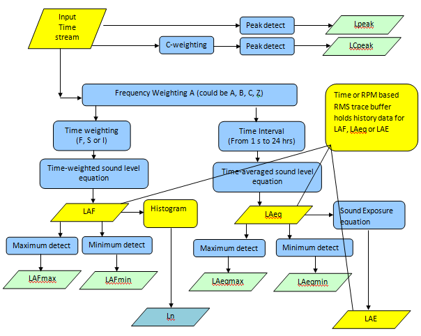
Figure 21. Sound level meter computation diagram
The SLM measurement is split into three paths after the digitized data arrives: one goes to frequency weighting A, B, C or Z and one goes to C weighting or no weighting. The peak detection is computed from the output of C weighting or no weighting. The output of frequency weighting (A, B, C or Z) is further split into two paths. The first will go to a time weighting function which is more or less equivalent to an exponential averaging mode to calculate LAF; the second path goes to a time averaging function, which is equivalent to a linear averaging mode to calculate Leq.
A list of symbols used by this instrument with A-weighted applied is provided in Table 3.
| Symbol of Measured Values | Description |
|---|---|
| LAF | A-weighted, F time-weighted sound level |
| LAfmax | Maximum A-weighted, F time-weighted sound level |
| LAfmin | Minimum A-weighted, F time-weighted sound level |
| LCpeak | Peak C sound level, greatest absolute instantaneous C-weighted sound pressure level |
| Lpeak | Peak sound level, greatest absolute instantaneous sound pressure level |
| LAeq | A-weighted, time-average sound level (equivalent continuous sound level) |
| LAeqmax | Maximum A-weighted, time-average sound level (equivalent continuous sound level) |
| LAeqmin | Minimum A-weighted, time-average sound level (equivalent continuous sound level) |
| LAE | A-weighted sound exposure level |
| LN (N = any integer between 0~100) |
Statistical Level general term |
| L1, L5, L50, L95.... | Statistical Levels with specific N values. The sound level exceeds this level 1, 5, 50 or 95 percent of the time for the duration of the measurement. |
Measurements Available to DSA in SLM Mode
There are two ways to view sound level measurements: instantaneous SLM measures and RMS history. Instantaneous SLM measures represent the most current value of the measurement.
RMS history not only shows the most current value, but also a record of historical values against time or RPM. Some of the measures allow only instantaneous values, others allow both.
The following measurement quantities are available to DSA in the measurement.
SLM Measures
The following SLM measures are available for real-time reading and can be saved as a data structure for future review.
Time Weighted Sound Levels
In DSA, time weighted sound level is the output of frequency-weighting and then time weighting filters. Time weighting serves an exponential averaging operator. The computation is illustrated in Figure 22.

Figure 22. Time weighting sound level computation and storage against RPM or Time
Table 4 shows the symbols for the time-weighted sound level.
| Symbol used for time weighted value | Frequency Weighting | ||||
|---|---|---|---|---|---|
| Z | A | B | C | ||
| Time Weighting | F(Fast) | LZF | LAF | LBF | LCF |
| S(Slow) | LZS | LAS | LBS | LCS | |
| I(Impulse) | LZI | LAI | LBI | LCI | |
| Custom | LZC | LAC | LBC | LCC | |
Time Averaged Sound Levels
In DSA, time averaged sound level is the output of frequency-weighting and then performing the time average operation. Time average serves a linear averaging operator. Figure 23 illustrates the computation.
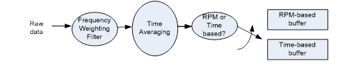
Figure 23. Time averaged sound level computation
The following table lists the symbols for time-average sound level. Frequency weighting can be selected as A, B, C or Z in the time averaging sound level measurement. The time interval for time averaging can be set to any value between 1 second and 24 hours.
| Frequency Weighting | Z | A | B | C |
|---|---|---|---|---|
| Symbol | Leq | Laeq | Lbeq | Lceq |
Peak Sound Level
Only C-weighted and un-weighted are available for peak sound level. This is required by the standards.
| Symbol | Lpeak | Lcpeak |
Sound Exposure Level
Sound exposure level and time-average sound level have the same frequency weighting and same time interval.
| Frequency Weighting | Z | A | B | C |
|---|---|---|---|---|
| Symbol | Leq | Laeq | Lbeq | Lceq |
Statistical Level: Value Reading
Any statistical level LN is the sound level which is exceeded for N% of the defined measurement duration.
| Symbols for LN, N = 1, 5, 50, 95 | L1 | L5 | L50 | L95 |
Input Channel Time Streams
The DSA developed by Crystal Instruments features time domain data that is always available in the form of long-time history. The user can view and record time signals. A limitation is that the sampling rate of the time signals cannot be arbitrarily changed. It is always set internally by the system based on the analysis frequency range.
RMS Trace of Weighted Level, Time Averaged Level or Sound Exposure
DSA records an RMS trace of the sound level. The user must choose between the time weighted level LAF, the equivalent time averaged level LAEQ, or sound exposure level LAE. Only one can be recorded at a time.
The RMS trace must be selected using Time or RMS as a variable during the CSA Editor stage.
Histogram of Time Weighting
DSA also records a signal containing a histogram of the dB values from the time weighted signal. This signal is used to compute the LN data.
Order Tracking is a general term that describes a collection of software functions used to analyze the mechanical dynamic behavior of rotating or reciprocating machinery for which the rotational speed can change over time. Unlike the power spectrum and other frequency-domain analysis standards where the changing variable is the frequency, Order Tracking functions present the data related to the variable rotating speed, i.e., RPM (revolution per minute).
The most useful measurements are order spectra and order tracks. An order spectrum gives the amplitude of the signal as a function of harmonic order of the rotation frequency. This means that a harmonic or sub-harmonic order component remains in the same analysis line independent of the speed of the machine.
The technique that observes the changes of any quantity vs. RPM is called tracking, as the rotation frequency is being tracked and used for analysis. Most of the dynamic forces exciting a machine are related to the rotation frequency so interpretation and diagnosis can thus be greatly simplified by use of order analysis.
Order tracks are simply the observations to the amplitude of the components with fundamental frequency or harmonics. It is a typical type of tracking. There are other types of tracking. For example, users can track the FFT-based PSD spectra, a fixed band, or an octave band.
The Crystal Instruments Order Tracking package enables the instrument to perform the following functions:
Process a tachometer signal and obtain a high-fidelity RPM measurement.
Measure the order spectra.
Measure the order tracks.
Measure the RPM FFT spectrum.
Measure the energy in fixed bands vs. RPM.
Measure the amplitude and phase of an order relative to the tachometer.
There are several different applications for order tracking. The following discussion covers several types.
The first application, often referred to as Run Up/Run Down, is used to evaluate the noise or vibration dynamic response when RPM is used as a changing variable. In this case, the RPM range can be very wide, from a few RPM to 10,000 RPM. Typical application tests are used in automotive or aircraft engines. The measurements can be any physical quantities such as sound, displacement, velocity, acceleration, torque, etc. The analysis measure can be the amplitude or the power of an order, the energy over a fixed frequency band, a bin of octave filter, etc. The phase information of the responses to tacho is less important in this type of application. In fact, the rotating element might be hidden inside a mechanical system. The primary result for this type of measurement is the magnitude of the responses vs. RPM.
The second application is rotating machine analysis that focuses on the measurement of displacement or velocity of the rotors during rotation. The instrument measures the amplitudes of specific orders and their relative phase to a reference signal. The phase is calculated relative to the tachometer input or a separate reference input. This application is commonly used for machine diagnosis and balancing. In this case, the RPM is stable or quasi-stable. Order tracking technology effectively increases the estimation accuracy of orders.
Order signals with phase are useful during the test of a rotating machine in the Run Up/Run Down process. This is often presented as a “Bode Plot”. The Bode Plot is a borrowed concept from control theory; it is a collection of Amplitude and Phase data over a changing speed range (e.g., Run Up or Coast Down). Some setup information depends on the rate of change for the RPM. The Run Up or Coast Down could take anywhere from a few minutes to a few hours (as required for a cold startup on a turbine). Other displays such as the orbit plot are useful as well.
The DSA includes the ability to measure RPM based octave analysis and sound levels. This feature is similar to order tracks except that spectra are recorded in octave bands with A, B, C or Z frequency weighting. This feature is included in the Acoustic Analysis and Sound Level Meter CSA templates instead of the Order Tracking Template. Refer to these sections for more details.
Tachometer Signal Processing and RPM Measurement
A tachometer (tacho) converts the angular velocity of a rotating shaft into an electrical signal, typically a voltage. It is common for calibrated instruments to provide a measurement of the shaft in units of revolutions per minute (RPM) or revolutions per second (RPS). Many modern rotating machines (electric motors, generators, pumps, turbines, IC engines, etc.) have integrated tachometers that can measure shaft angular velocity. An example of an optical tachometer is shown in Figure 24.

Figure 24. Optical tachometer setup
The goal of tacho signal processing is to obtain a clean and stable RPM reading. The tacho signal must be carefully processed to provide a base of tracking. Any order tracking results can only be thought of as being as accurate as the tachometer signals that were used to estimate the instantaneous frequency of the order in the analysis process. If the quality of the tachometer channel is poor, the results from all other channels will be poor or even unreliable.
In old analog methods, tacho channels were conditioned with a tracking ratio tuner containing a phase lock loop. The disadvantage of this method is the limited slew rate and the use of complex hardware. Various digital tacho processing methods have been developed to overcome these limitations.
From a hardware design perspective, there are two options to implement a tacho input channel: use a dedicated tacho channel with a digital counter or use an analog input channel.
Dedicated Tacho Channel Using Counter
Many users prefer a dedicated tacho channel without an A/D converter. This hardware approach contains its own tacho clock which runs at a much higher speed, typically in MHz. This tacho hardware also contains special counters which maintain a continuous counter reading to avoid skipping any triggered cycles of the tacho signal. An available option allows these counters to "average" several tacho periods for cases when the input tacho frequency is very high.
Using Analog Input Channel
Alternatively, some systems use an analog input data channel as a tacho channel. In this case, the tacho clock is actually the sample rate of the data channels. This sample rate usually limits the tacho frequency range since the tacho range is now set by the input data frequency range requirement. In addition, due to the "frame processing" nature of some not-so-well designed input sampling processes, some instruments may be limited to how they acquire the tacho signal. This restriction usually means they get several tacho cycles in every data frame. The result is often an "averaged" value, which is okay unless the tacho signal is changing frequency during the data frame event, which is often the case.
The advancements of electronics and the lowered price of electronic components has decreased cost concerns. The approach of a dedicated tacho channel with a digital counter, without A/D, may or may not be the best choice.
The DSA can use any data channel as a tacho channel. Channel 1 is usually designated as the tacho to facilitate a simple interface design. The special hardware circuitry allows this data channel to sample at the highest possible sampling rate while the data input channel is used as a tacho measurement. In other words, the tacho speed measurement accuracy depends on the current range of the analysis frequency. This technique has several obvious advantages:
The time domain signal of the tacho input is transformed by the A/D converter into a digital signal. Users can observe the pulse trains of the tacho signal and arbitrarily set the threshold.
Accurate phase information can be obtained relative to each data channel because the tacho channel, which is fed by high frequency sampling counter, is synchronized with data channels.
The RPM estimation is not influenced by the current data sampling rate.
High Pulse per Rev
Pulse per Rev is defined as the number of pulses per revolution. Pulse per Rev. must be defined by the user so the instrument can calculate the reference frequency of tacho using tacho frequency. The relationship is:
Tacho Reference Frequency = (Tacho Frequency)/(Pulse per Rev)

Figure 25. Tach pulse, pulse period and revolution period
The Pulses per Rev is simply 1 in most rotor tests, especially in balancing. Other cases such as flywheel or geared data measurement can have the Pulses per Rev as high as in the hundreds. A dedicated tacho channel with a high speed counter might work better to address this situation.
The CoCo-90 can use any data channel as a tacho input and features a dedicated installed tacho channel to measure a high-speed RPM, deal with high Pulses/Rev, or perform as a digital TTL trigger. The counter speed is about 25 MHz. This second choice provides a more versatile solution to users for their applications.
The special tacho hardware design in the DSA system with Order Tracking offers the most accurate possible approach for performing a wide range of real-time machinery-related vibration and noise analysis.
Pulse Detection
A good tacho processing device should provide users with a visual of the tacho signal in its original time waveform and set the Pulse per Rev., the threshold of pulse detection. This will help set up the tachometer and quickly diagnose any problems. DSA hardware provides users with a special display window to conveniently switch between the RPM trace and the tacho original time waveform displays. The pulse detection threshold is easily controlled with the Up/Down buttons.
Order Tracks and Order Spectrum
Knowledge of the rotating speed allows presentation of measurement results in the angle and order domains, corresponding to the time and frequency domains. An order is a frequency normalized with some reference frequency, e.g. the shaft frequency. This means that the order of a vibration component in the order spectrum indicates the number of vibration cycles per shaft revolution. The magnitude, which can be measured using EUpk, EUrms, or EUrms2, of an order is the measurement extracted through a tracking filter with the center frequency located at this frequency. Multiple measurements of a range of orders will construct what is called an Order Spectrum. An order power spectrum measurement produces a quantitative description of the amplitude, or power, of the orders in a signal. It provides a useful display of all order components in a signal. This can help users locate significant orders and compare the level of different order components.
Two methods to perform rotationally coherent sampling are phase-locked frequency multipliers and digital re-sampling. Phase-locked frequency multipliers were mainly used in early work. They generate sampling pulses based on a rotational reference signal. These sampling pulses control the sampling process. Note that the sampling frequency will depend on the rotational speed, and thus an adjustable anti-aliasing filter is needed. This complicates the method considerably. In the digital re-sampling technique, the time signal is conventionally sampled together with some rotational reference signal. The time signal is then digitally re-sampled to the angle domain by interpolation techniques. The rotational reference signal can be acquired with a tachometer or an incremental pulse encoder.
Figure 26 conceptually illustrates how angle data re-sampling can be used to analyze vibrations from an engine during start up. Once the signal has been transformed into its angle domain, the FFT can be applied to analyze the order spectrum of the vibrations.

Figure 26. Angular data re-sampling of a chip signal
The last plot in the figure illustrates that the sampling rate will be determined by both instantaneous tacho speed and the required analysis frequency range.
The DSA system computes the order tracks and order spectrum with a proprietary technology that combines digital re-sampling with data decimation and interpolation in addition to DFT and FFT calculations.
Three measurements can be generated from an order tracking computation. The 3D RPM Order Spectrum is simply a 3-dimensional view of the other two types of measurement. Another way to visualize these types of plots is that the order spectrum is a cross section of the 3D plot along a fixed RPM value while the order track is a cross section along a fixed order number. Their relationships are illustrated in Figure 27, 28, and 29:

Figure 27. Typical order tracks
Figure 28. Typical order spectrum

Figure 29. Typical 3D order track waterfall plot
An important concept introduced in this section is delta order, ΔOrder. In the FFT based frequency spectrum analysis, the frequency span and frequency resolution are fixed. The capability of discriminating frequency components is equal in both the low and high frequency. In rotating machine analysis, it is desirable to have better analysis resolution in the low frequency rather than in the high frequency. For example, if the rotating speed is at 60 RPM, users will definitely care if the instrument can tell the difference between 1 Hz (order 1) and 2 Hz (order 2). On the contrary, if the rotating speed is at 6000 RPM, the user probably will not care if the instrument can discriminate the measurement between 100 Hz (order 1) and 101 Hz.
The digital re-sampling technique extracts the order tracks and order spectrum based on a filter with equal ΔOrder instead of equal ΔFrequency. The concept is illustrated in the following figure.

Figure 30. Comparison of constant band tracking and digital re-sampling method
The left side of Figure 30 shows the ΔFrequency of the tracking filter will be fixed when the order tracks are extracted using a conventional FFT method with fixed resolution. The right side shows that if the order tracks are extracted using digital re-sampling, the ΔFrequency tracking filter will be increased proportionally with the RPM. Obviously, digital re-sampling is the more desirable method when extracting the measurement of orders.
RPM Frequency Spectrum
While the order tracks and order spectra are developed to analyze the characteristics of the system on the order space, the measures of fixed bands are also helpful for analysis. Like the RMS time trace for a given frequency band with time as variable, the RMS trace can be extracted for a given frequency band with RPM as the independent variable. This is simply called an RPM Spectrum. An RPM Spectrum can be described as a 3D waterfall as illustrated in Figure 31.
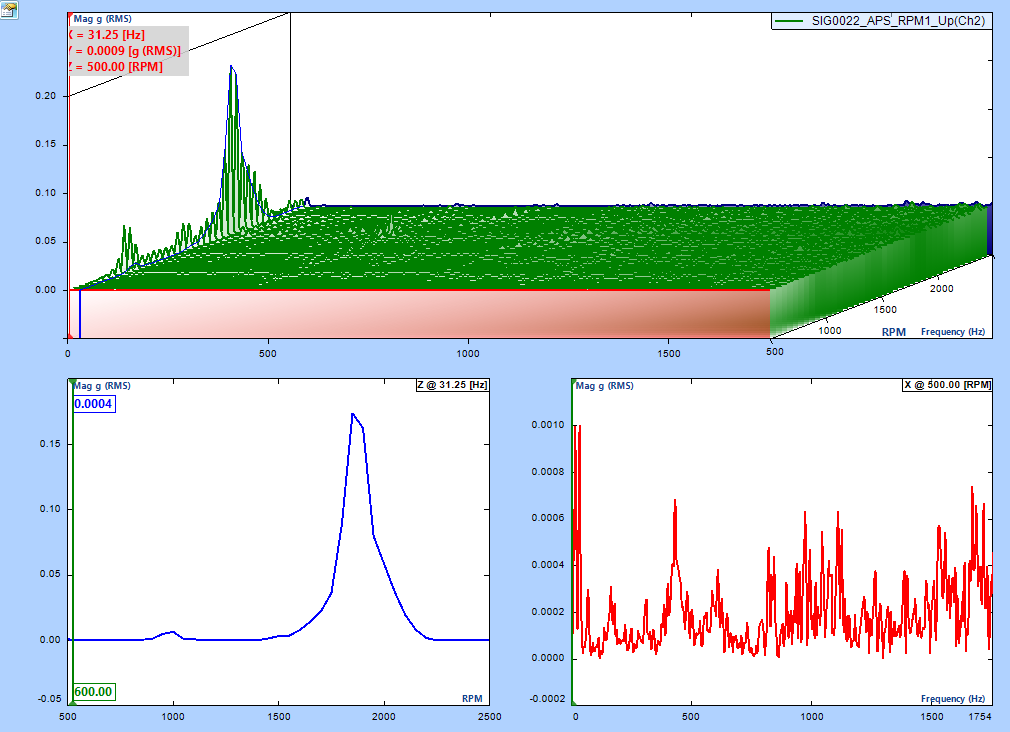
Figure 31. Typical RPM spectrum waterfall plot
The horizontal axis of the 3D RPM Spectrum is frequency. The Z axis is RPM, and the measurement unit is usually EUrms2 or EUrms. A color map can also be used to describe the magnitude of the whole range as shown demonstrated in Figure 32.
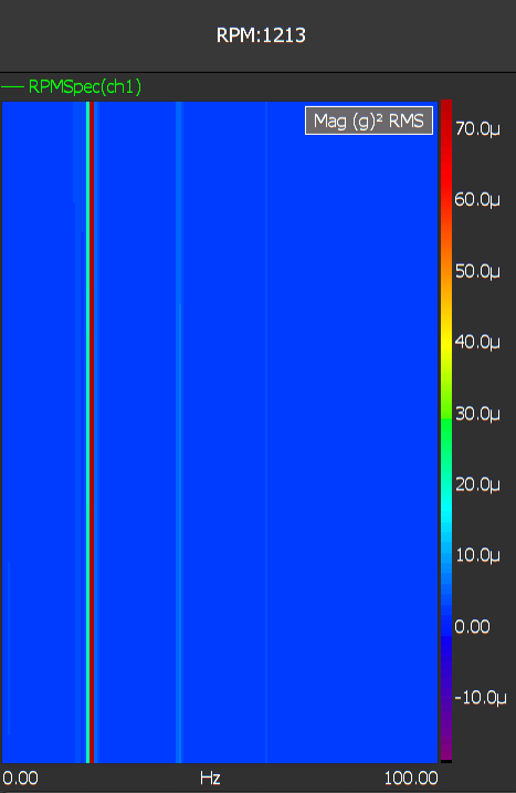
Figure 32. Color map of an RPM spectrum
The instrument can use a 3D RPM frequency spectrum to extract the total energy over a fixed frequency band and plot it with RPM as the independent variable. This is called a Fixed Band RPM Spectrum as shown in Figure 33.

Figure 33. Fixed band RPM spectrum
An engineering measurement unit of Fixed Band RPM Spectrum is expressed as EUrmsrms2 or EUrms, which represents the total power measured in a fixed band versus the rotating speed change. This data is particularly useful to watch the total magnitude in a resonance area when the rotating speed of the shaft is changing. Users can define the frequency band around the resonant frequency and perform a run up/down test. Both order tracking and order spectrum cannot extract the response magnitude of the resonance as accurately as a fixed band RPM spectrum because the bandwidth of the tracking filter of order tracking is not explicitly controlled.
Overall Level Measurement
In order tracking, it is important to monitor the overall RMS level or power level of the measurement versus RPM. The overall level is a good reference for comparison with other signals such as order tracks or fixed band RPM spectrum.
The overall level can be expressed in units of RMS (EUrms) or power (EUrms2). The horizontal axis is RPM. Figure 34 depicts a typical overall level display.

Figure 34. Overall RMS level plot
Raw Data Time Streams
Many other order tracking software products limit their users to conducting real-time order tracking analysis or recording data before post processing the order tracks. The DSA is a high performance data recorder in addition to a real time analyzer and can perform both tasks at the same time. Continuous time streams of each input channel are always available even while order track data is computed.
Order Tracks with Phase
The Phase in Rotating Machine Analysis
Analyzing order magnitude and phase can help users detect mechanical faults directly since many mechanical faults are associated with certain orders. For example, a strong first order magnitude indicates imbalance in most cases. Analyzing the first order magnitude can help identify the imbalance. Moreover, the magnitude and phase of the first order can help the user to correct the imbalance by adding weights on the appropriate rotor positions. Fixing imbalance problems requires phase information of order tracks. A list of vibration sources from a rotating machine are provided in the following table:
| Order | Source of problem |
|---|---|
| 0.05X~0.35X | Diffuser Stall |
| 0.43X~0.49X | Instability |
| 0.5X | Rubbing |
| 0.65X~0.95X | Impeller Stall |
| 1X | Imbalance |
| 1X+2X | Misalignment |
| (#Vane)X | Vane/Volute gap |
| (#Blades)X | Blade/Diffuser Gap |
As previously discussed, an order track is the measurement taken for an order, i.e., normalized frequency, versus RPM. The phase information of order tracks is not important in most applications of engine related testing. In rotating machine analysis, the phase of the signal is vitally important.
Phase is a relative measurement quantity and can only be measured with a pair of signals. It indicates the time delay at a certain frequency between two signals. The phase value can be translated into the difference of relative angle, relative position, or propagation time if additional information is given. When referring to the phase information of one signal, we imply its phase is relative to a reference signal that was mentioned in context.
In rotating machine analysis, the phase of the first order of the rotor can be directly mapped to an angular difference between a signal and the reference signal. The reference signal can be another channel of measurement or the tachometer signal.
The phase difference between two waveforms is often called a phase shift or phase delay. A phase shift of 360 degrees is a time delay of one cycle or one period of the wave, which actually amounts to no phase shift at all. A phase shift of 90 degrees is a 1/4 shift of the wave period. Phase shift may be considered positive or negative and one waveform can be delayed or advanced relative to another one. These conditions are called phase lag and phase lead respectively.
An example of this is the phase of an imbalance component in a rotor with reference to a fixed point on the rotor, such as a key way. To measure this phase, a trigger-pulse must be generated from a certain reference point on the shaft. This trigger can be generated by a tachometer or an optical or magnetic probe that senses a discontinuity on the rotor and is sometimes called a "tach" pulse.
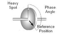
Figure 35. Shaft phase wrt. Reference tacho
A zero degree phase delay at a frequency can be depicted as a series of pulses overlaid with a sine wave where the pulse edge is located exactly in peak position of the sine wave.

Figure 36. Schematic of tacho pulse and vibration signal
Figure 36 shows a section of the tacho signal on its own and then overlaid on the vibration signal. The tacho signal in this example crosses the vibration signal at exactly the same point on each cycle. If the phase of the vibration signal were to change then its position relative to the tacho pulse would also change. Extracting the first order modulus and phase, as before, produces the curves shown in Figure 37 and Figure 38. The phase is now constant near -60o as it should be for such a signal. If the rotating period of the signal is about 20 ms, -60o corresponds to a 20*60/360 = 3.3 ms delay.
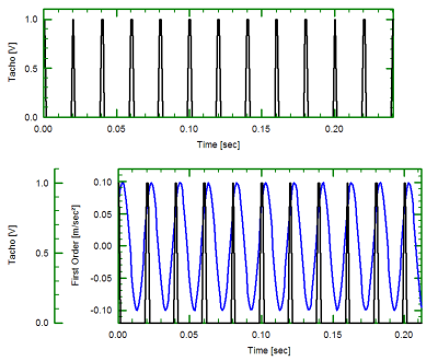
Figure 37. First order modulus extraction

Figure 38. First order modulus and phase extraction
The phase measurement at higher orders will have a similar physical interpretation although they are difficult to comprehend intuitively.
It must be noted that the order tracks with phase, otherwise known as Complex Order Tracks, are not regular complex signals as frequency response or cross spectrum. These are actually auto-spectra with assigned phase. These synthesized signals can certainly be viewed as a complex signal using tools such as Bode, polar, and orbit plot diagrams. Users must keep in mind that the magnitude and phase of a complex order track are calculated separately.
The following sections will present how the order tracks with phase can be presented graphically using the Bode, polar, and orbit plot.
Bode Plot
The term Bode plot is borrowed from the field of control theory, referring to a plot of magnitude and phase angle between the input and output verses frequency of a control system. Many in the rotating machine vibration industry have adopted this term to describe the steady-state vibration response amplitude and phase angle versus rotational speed (RPM). It turns out that the Bode plot is the best way to describe order tracks with phase. Bode plots are typically used for transient analysis in both start-up and coast-down conditions. A Bode plot can help to identify the resonance speed of a rotor or examine the rotor dynamics on an order basis. A typical Bode plot for an order track is shown in Figure 39.
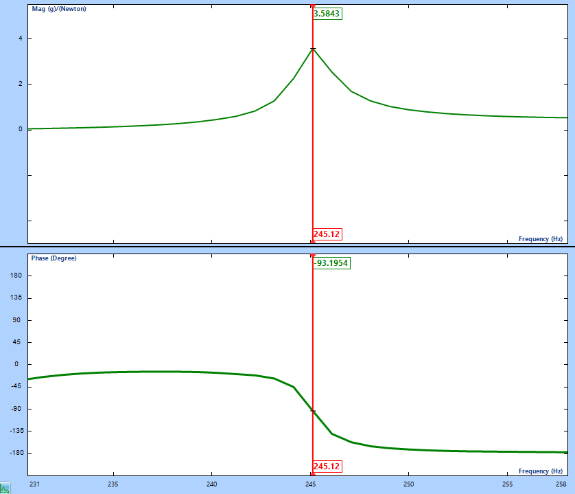
Figure 39. Bode plot
The Bode plot in the DSA system can show one or multiple tracks after the order tracks are acquired with their phase information.
Polar Plot
The polar plot is another useful tool to view the order tracks for both amplitude and phase information. A polar plot draws the amplitude and phase on a polar coordinate. A typical polar plot is shown in Figure 40.
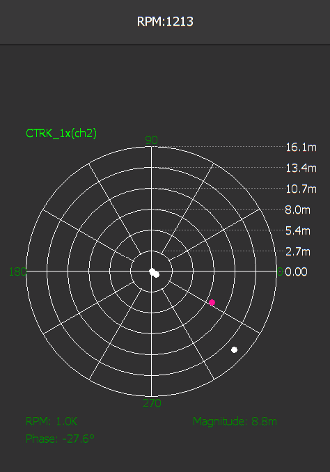
Figure 40. Polar plot shows magnitude and phase on a polar axis
A dot shows the current order track value in the polar plot. The distance between the dot and the center indicates the magnitude of the order track while the angle corresponds to the phase measurement. The polar plot only shows the instantaneous measurement. It cannot keep the history versus RPM.
The polar plot is often used to visually indicate the imbalance of the rotor. Polar plots and Bode plots are often combined to describe the rotating speed vector signal locus during speed changes. A Bode plot provides excellent change visibility with respect to speed, while the polar plot shows improved phase variation resolution.
Orbit Display
The orbit display uses two data channels in the time domain. The signals from two channels are drawn on an X and Y plane to display the shaft position change versus angle of rotation. Orbit displays produce a two-dimensional visual picture of the motion of a rotating shaft.
A well-balanced shaft with no movement in any direction and would produce a dot in the middle of the plot. The shaft movement can indicate the vibration source. (e.g., a lot of up/down movement may indicate the machine feet are not bolted down tightly enough.)
To create an orbit plot, take a dual channel simultaneous measurement to capture data at the horizontal and vertical axes at the same time. The displacement or acceleration sensors must be placed 90° apart from each other.
An orbit display uses a pair of measurements in time domain. It does not need the order tracking technique.
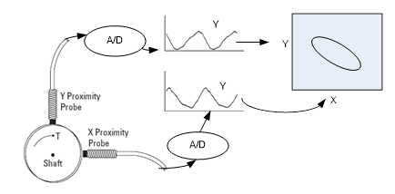
Figure 41. Procedure for an Orbit plot
The orbit display is like the polar display in that it only displays the instantaneous status at the current RPM. In theory, the orbit display does not need a tachometer or another reference signal because X and Y reference each other.
Summary
The order tracks with phase can be presented visually using the Bode, polar, and orbit plots. These effective tools are used for rotating machine analysis. Bode plot is mostly used in the Run Up/Coast Down process. Polar plot and orbit, which only show the instantaneous status of an order at current RPM, are adequate for applications at steady or quasi-steady rotating speed such as dynamic balancing.
A Shock Response Spectrum (SRS) is a graphical representation of an arbitrary transient acceleration input, such as shock in terms of how a Single Degree of Freedom (SDOF) system (i.e., a mass on a spring and damper) responds to that input. It shows the peak acceleration response of an infinite number of SDOFs, each of which have different natural frequencies. Acceleration response amplitude is represented on the vertical axis, and natural frequency of any given SDOF is shown on the horizontal axis.
A SRS is generated from a shock waveform using the following process:
Select a damping ratio for the SRS
Assume a hypothetical Single Degree of Freedom System (SDOF), with a damped natural frequency of x Hz
Calculate (by time base simulation or something more subtle) the maximum instantaneous absolute acceleration experienced by the mass element of the SDOFs at any time during (or after) exposure to the shock in question. Plot this in g's (g's are standard but pick any desired unit of acceleration) against the frequency (x) of the hypothetical system.
Repeat steps 2 and 3 for other values of X, e.g., logarithmically up to 1000x.
The resulting plot of peak acceleration vs. test system frequency is called a Shock Response Spectrum, or SRS. This process is depicted in Figure 42.
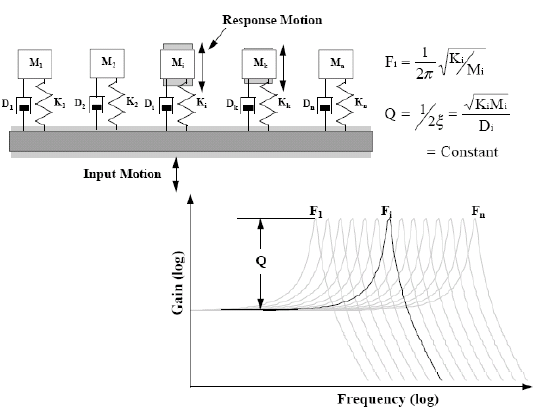
Figure 42. Illustration of multi-degree of freedom system model used to compute SRS
A SDOF mechanical system consists of the following components:
Mass, with its value represented by the variable, M
Spring, with its stiffness represented by the variable, K
Damper, with its damping coefficient represented by the variable C.
The resonance frequency, Fi, and the critical damping factor, ζ, characterize a SDOF system, where:
Fi= 1/2π √(K/M)
ζ= c/(2√KM)
For a light damping ratio where ζ is less than or equal to 0.05, the peak value of the frequency response occurs in the immediate vicinity of Fi and is given by the following equation, where Q is the quality factor:
Q= 1/2ζ
Any transient waveform can be presented as an SRS, but the relationship is not unique; many different transient waveforms can produce the same SRS (something one can take advantage of through a process called "Shock Synthesis"). The SRS does not contain all the information about the transient waveform from which it was created because it only tracks the peak instantaneous accelerations.
Different damping ratios produce different SRSs for the same shock waveform. Zero damping will produce a maximum response. Very high damping produces a very flat SRS. The level of damping is demonstrated by the "quality factor", Q which can also be thought of transmissibility in a sinusoidal vibration case. A damping ratio of 5% results in a Q of 10. An SRS plot is incomplete if it does not specify the assumed Q or damping ratio value.
Frequency Spacing of SRS Bins
The SRS spectrum usually consists of multiple bins distributed evenly in the logarithmic frequency scale. The frequency distribution can be defined by two numbers: a reference frequency and the fractional octave number, such as 1/1, 1/3 or 1/6.
An octave is a doubling of frequency. For example, frequencies of 250 Hz and 500 Hz are one octave apart, as are frequencies of 1 kHz and 2 kHz.

Figure 43. Full octave filter shape
The proportional bandwidth property will divide the frequency information uniformly over a log scale. It is very useful in analyzing a variety of natural systems. For example, the human response to noise and vibration is very non-linear and many mechanical systems have a behavior that is best characterized by a proportional bandwidth analysis.
To gain finer frequency resolution, the frequency range can be divided into proportional bandwidths that are a fraction of an octave. For example, with 1/3 octave spacing, there are 3 SDOF filters per octave. In general, for 1/N fraction octave, there are N band pass filters per octave such that:
fj+1 = fj * 21/N
where 1/N is called the fractional octave number. The reference frequency fr is simply a selected frequency fj. All other frequencies of SDOF filters reference this frequency. When the reference frequency and the fractional octave number are defined, the frequency distribution over the whole frequency range is determined.
SRS Measurement Quantities
Measurement quantities available to the DSA SRS test are: time stream of each channel (raw data), block captured time signals and three SRS of each channel.
Time streams: this is the same as any other applications on the DSA. Time streams are always available for viewing and recording . It is a very useful tool to observe whether the input signals are in the valid range. The recorded sine wave can be used for further post-processing. In DSA, the time streams are often denoted as ch1, ch2 etc.
Block time signals: These are block captured signals that are used for SRS analysis. Acquisition Mode will control how the block time signals are acquired.
SRS: Shock Response Spectra will be calculated for each block time signals. The engineering unit of the spectrum is determined by the sensor used by the input channel. In DSA, the spectra are often denoted as three types: Maximum Positive spectrum; Maximum Negative spectrum and Maximum-Maximum spectrum.
Maximum Positive Spectrum: This is the largest positive response due to the transient input, without reference to the duration of the input.
Maximum Negative Spectrum: This is the largest negative response due to the transient input, without reference to the duration of the input.
Maximax Spectrum: this is the enveloge of the absolute values of the positive and negative spectra. It is the most often used SRS type. The log-log Maximax is the universally accepted format for SRS presentation.
Other common SRS measures include Primiary SRS, Residue SRS and Composite SRS. The DSA only calculates the Composite SRS.
Automated limit testing allows engineers and technicians to set up a pass/fail measurement on any measured signal. This feature automates the process of determining whether an acquired signal meets, or is within a given set of criteria.
A limit test typically consists of comparing a waveform to upper and lower boundaries which the measured waveform must not cross. These boundaries are typically defined by the user to specify a tolerance band around a waveform. If any part of the waveform falls outside the limit, the software returns a failure message and the location of the failure on the waveform.
Application Examples
A common example for automated testing is related to structural testing. When excited, a structure will resonate at its natural frequencies. Structures can be excited through impact or by other means. Structural defects can result in a shift in resonant peaks. Therefore, in structural tests, frequency ‘alarms’ are used to monitor the frequency response in areas of spectral interest.
Another example of automated testing is related to rotating machinery. Rotating or moving assemblies produce vibration and noise patterns that can be examined to identify the fingerprint of ‘good quality.’ Product defects will cause additional spectral peaks, or changes in peak levels. Therefore, in ‘self-excited’ product testing, ‘level alarms’, which can be set to trigger on peak or RMS values, are placed around the areas of spectral interest. Unwanted signals, from background noise, are therefore ignored.
Testing Limit Signals and Testing Schedule
Automated testing can be performed on a wide variety of signals including a time domain capture, an auto-power spectrum, an octave spectrum, an order track signal or a frequency response. The DSA instrument compares the limits to the live measured signal in real-time, after every single frame of measurement. If the limits are exceeded, the DSA takes the appropriate actions based on the user setup.
An upper and or lower limit can be applied to a signal to be tested. Limit signals are constructed by defining breakpoints. A breakpoint is controlled by a pair of X/Y values. Figure 44 shows a typical automated test limit signal with 4 breakpoints.
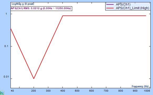
Figure 44. Typical automated test limit signal with 4 breakpoints for Auto Power Spectra on an input channel
To automatically control the limit checking test, a testing schedule is developed for DSA. The testing schedule defines the various operations to automate the process. For example, the testing schedule can tell the instrument when the limit checking will be turned on, when it will be turned off, and the duration it will be conducted.
To record the events of the test a Testing Log and a summary report are needed. The Testing Log records the important events, including whether the limits are exceeded, in chronicle order. The Summary Report provides the status of limiting check since the last time the test was started.
When the limit signal is exceeded, a user defined limit alarm event will be triggered. This can include an audible beep, save signals, send messages and more.
To summarize, an automated limit checking test requires the following building blocks:
At least one test signal
At least one limit signal applied to the measured signals
A testing schedule
A testing log and summary report
A setup for the limit alarm events
Figure 45 illustrates the automated testing process.

Figure 45. Illustration of automatic testing process
Test Signals: Any block signal can be used for testing. The test signals are typically time captured blocks, auto power spectra, frequency response, octave spectra or order tracks. Time streams are not used for limiting tests.
Limit Signals: Limit signals including upper and/or lower limits are defined in the CSA Editor. Limit signals are applied to testing signals. Up to a maximum of 64 segments can be defined for each limit signal. The maximum number of limit signals is 64.
Testing Schedule: The testing schedule automatically controls the test using an event driven process. Multiple testing schedules can be developed and one is executed at a time. Testing schedule event entries include: Loop/End-Loop, Set Sampling Rate, Set All Input Mode, Run Duration, Hold, Limit Check on, Limit Check off, Start Recording, Stop Recording, Save Signals, Turn Signal Source On and Turn Signal Source Off.
Testing Log: A log file is automatically created for each run of the schedule to record major events.
Limit Check Alarm Event Setup: Events include an audible beep from the DSA, screen flashing, entry into the Testing Log, send message to host PC via EDM software and Save Signals.
When a limit is exceeded, the predefined events are triggered. For example, the DSA may beep, flash the screen, save signals to a storage device, or send a message to the host PC.
Networked DSA Used for Automated Test
DSA uses an Ethernet network interface with a unique advantage of allowing multiple units to connect remotely. This is particularly useful for vibration monitoring or production testing with requirements for long distance access. (Figure 46)
Figure 46. Remote operation for multiple CoCo DSA units with automated testing
When multiple DSA units are managed through the EDM software, the host computer can record or react to the alarm events from each remote DSA unit.
Real Time Digital Filters is a powerful built-in DSA analysis tool that can filter a measured signal in real time and then apply the FFT and time based analysis. Users can precisely define the filter characteristics to meet a specific application. The filter definition is performed in the EDM software and is included in the CSA file that is downloaded to the CoCo. This capability in a small portable unit makes the DSA a very powerful analysis tool.
Some users may want to view the energy distribution over time for a specific band of frequencies instead of the entire frequency spectrum from zero to the maximum sampling rate. This is accomplished by creating a band-pass filter and then applying an RMS estimator to the output of the filter. Figure 47 shows the graphical representation of this process which is used to define the real time filter in the EDM software. The icon on the left, CH1 represents the native measured time stream. It is connected to an IIR Filter which computes a signal labelled iirfilter (ch1) and is connected to an RMS estimator. The output of the RMS estimator is a signal labelled rms(iirfilter(ch1)). (Figure 47) The EDM software is discussed in more detail later.

Figure 47. Example real time digital filter application
Another example users may want to view separately is the frequency energy over 100 Hz to 200 Hz and 1000 Hz to 2000 Hz. This is accomplished by deriving two output streams from the native channel 1 and then applying the band-pass filter to each path as shown in Figure 48.

Figure 48. Digital real time filter example with two output streams
In another example, a user may want to view the very fast time characteristics of a channel at a high frequency and the same channel at a very low sampling rate. This is accomplished by applying a decimation filter to the native time stream as shown in Figure 49. The native channel time stream is split into two streams to record the signal from the same channel at both high and lower sampling rates.

Figure 49. Example computing high and low sampling rate with a decimation filter
The Real Time Digital Filters option includes three types of digital filters: FIR, IIR and decimation filters. For FIR and IIR filters, users can specify low-pass, high-pass, band-pass or band-stop types with several different methods. This chapter first explains the filter design theory and then introduces the operations within the CSA Editor and DSA hardware.
Real Time Filter implementation can be divided into two steps: first to define the filter in the EDM software and second to download and run the CSA on the DSA hardware.
Users can design filters based on certain criteria such as cut-off frequency, pass band ripple, attenuation level and more. The EDM software walks users through this process. The outcome of this design process is simply a number of filter coefficients that represent the filter which are included in a CSA. The software will upload the CSA including the filter coefficients to the DSA hardware.
Run the CSA after the filter is defined and the coefficients are downloaded to the DSA hardware. When the DSA is running, the filter coefficients created in the filter design process will be used. The time streams will pass through the filters and generate new time stream signals.
The goal of filter design is to calculate a series of filter coefficients, also known as “taps” based on the user specified criteria. The criteria are often described by the following variables:
Number of filter coefficients: also known as the order of the filter. The filter order defines the number of required coefficients to define the filter. A lower order filter consists of a fewer number of coefficients. A low order filter responds relatively faster than a higher order filter, with less time lag in the output of the filter.
Cutoff frequencies: Low pass or high pass filters only require one cutoff frequency. Band pass or band stop filters require two cutoff frequencies to fully define the filter shape. Figure 50 shows a typical band pass filter design with the two cutoff frequencies set to approximately 0.1 and 0.2 Hz as indicated by the blue and yellow vertical lines.
Attenuation of stop band in dB: This defines how much of the input signal is cut out of the output at the rejected frequencies. In theory the higher the attenuation the better. In Figure 50 the stop band attenuation is > 40 dB as seen from the highest side lobe just below 0.25 Hz.
Pass band ripple: Ripple is an unavoidable characteristic in a digital filter. It refers to the fluctuation in the filter shape at transition frequencies. If a very flat filter is required then it can be specified by choosing a very low ripple. Figure 50 shows ripple in the stop band and no ripple is evident in the pass band. Ideally the pass band should be very flat, and some ripple is tolerable in the stop band.
Width of transition bands: This refers to the filter shape between a band pass and a band stop region. Ideally this transition band should be very small. However, a very narrow transitional band requires a higher order filter which affects the filter response time and can also affect ripple. In Figure 50 the transition bands are between 0.05 to 0.1 and 0.2 to 0.25.

Figure 50. Filter design shows cutoff frequencies, ripple, band stop attenuation
Most cases of filter design include making tradeoffs between minimizing the filter order, ripple, transition band width, and response time. Not all variables can be satisfied at the same time. Filter design can be an iterative process and experience is helpful.
FIR Real Time Digital Filters
Finite Impulse Response (FIR) filters have the distinctive trait that their impulse response lasts for a finite duration of time as opposed to an Infinite Impulse Response (IIR) filter with an impulse response that lasts for an infinite duration. This trait is due to the lack of feedback paths in the FIR filter. FIR filters offer several advantages over IIR filters:
Completely constant group delay throughout the frequency spectrum. Group delay refers to the time delay between a signal going into the filter and when it comes out. Constant group delay means that an input signal will come out of the filter with all parts delayed the same amount with no distortion.
Complete stability at all frequencies regardless of the size of the filter.
FIR filters also have some disadvantages as well:
The frequency response is not as easily defined as it is with IIR filters
The number of coefficients required to meet a frequency specification may be far larger than that required for IIR filters.
DSA allows up to 128 taps (orders) for a real-time FIR filter.
A digital filter can be understood by considering the difference equation which defines how the input signal is related to the output signal as
y[n] = b0x[n] + b1x[n-1] +...+ bNx[n-N]
where x[n] is the current input signal sample, x[n-1] is the previous signal sample and x[n-N] is the last sample in the series. The series multiplies the most recent N+1 samples with the N+1 filter coefficients. y[n] is the current output signal and bi are the filter coefficients. The number N is known as the filter order; an Nth-order filter has (N + 1) terms on the right-hand side and N+1 filter coefficients also referred to as “taps”.
This equation illustrates why a higher order filter has a slower response time. It takes more samples and therefore more time for an event to work its way through the series until the output is no longer affected by the event as compared to a lower order filter with fewer coefficients.
The previous equation can also be expressed as a convolution of the filter coefficients and the input signal.

The Impulse Response of the filter shows how the historical data affects the current filtered value. The longer the impulse response, the farther the old data will affect the current filtered value. To find the impulse response set the following:
x[n] = δ[n]
where δ[n] is the Kronecker delta impulse. The equation below shows that the impulse response for an FIR filter is simply the set of coefficients bn, as follows
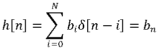
for n=0 to N
FIR filters are clearly stable, since the output is a sum of a finite number of finite multiples of the input values, so can be no greater than

times the largest value appearing in the input.
Data Windows FIR Filter Design
In the academic world, hundreds of methods are available to design an FIR filter to meet various criteria. EDM software includes the most popular filter design methods: Data Window and Remez. Both methods are discussed below.
The Data Window FIR Filter Design method is the easiest to understand. The name "Window" comes from the fact that these filters are created by scaling a sinc (SIN(X)/X) function with a window such as a Hanning, Flat Top, etc. to produce the desired frequency effect.
A data window FIR filter is generated by starting with an ideal “brick-wall” shaped filter, which is a filter with vertical edges, or zero transition band width as shown on the left in Figure 51. The brick-wall filter is specified by cutoff frequencies and has a band pass amplitude of 1 and a stop band amplitude of zero. The problem with the ideal brick-wall filter is that the time response oscillates forever, and it requires an infinite number of filter coefficients. This ideal filter can be modified by applying a data window to force the time response to decay in a finite time. As a result, this degrades the shape of the ideal brick-wall filter performance. It introduces ripple, increases the transition band width, and increases the stop band attenuation. However, it allows the filter to be defined by a finite number of filter coefficients. The filter performance can be modified by using different data windowing functions and making the tradeoff between filter order and response time. The user must choose these settings during the filter design.

Figure 51. Sinc function is the Fourier transform of a square shape
Figure 52 through Figure 58 shows a comparison of different data window choices for the same filter settings. In all cases the low and high cutoff frequencies are 0.1 and 0.2 relative to the sampling frequency. The number of filter taps is 51.

Figure 52. Hanning window method

Figure 53. Hamming window method

Figure 54. Flattop window method
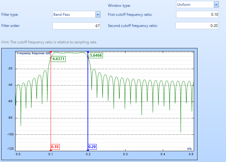
Figure 55. Uniform window method
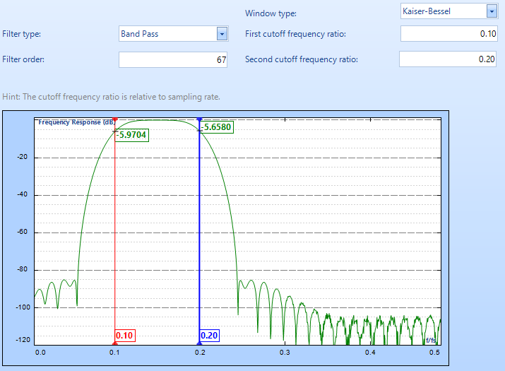
Figure 56. Kaiser Bessel window method

Figure 57. Blackman window method
As shown in the figures, different window methods produce a different filter performance, i.e., different attenuation of the main lobe and side lobes. The best data window choice depends on the specific application. Refer to the Basic Spectral Analysis section for a comparison of windowing functions.
Remez Filter Design
The Remez Filter is a different method for designing an FIR filter. It is more computationally intensive than the data window method. A Remez filter is generated with iterative error-reducing algorithms designed to reduce the pass-band error. In addition to allowing stop band ratio and frequency definition, the Remez filter allows the "Ripple Ratio" to be defined as a user specified parameter.
Figure 58 shows an example of a filter design using the Remez method provided by EDM software. The low and high cutoff frequencies are 0.1 and 0.2 relative to the sampling frequency. The number of filter taps is 51.

Figure 58. Ramez FIR filter design dialog
The software is intelligent enough to automatically calculate the total FIR filter length based on these criteria. For example, if the user asks for very high attention, very small ripple or a very sharp transition band, the filter length will be very high. The user must make tradeoffs between these parameters so that an appropriate filter length can be generated and used.
IIR Real Time Digital Filters
The impulse response from Infinite impulse response (IIR) filters decays very slowly but theoretically lasts forever. This is due to the fact that the filter input includes the measured signal and the filter output to create a feedback path resulting in an infinite impulse duration. This is in contrast to finite impulse response filters (FIR) which have fixed-duration impulse responses.
The design procedures for IIR filters is somewhat more complicated than FIR filter design because there is no direct design method like the data window method for FIR filters. Instead IIR filters are typically designed by starting with an ideal analog filter in terms of the frequency response characteristics such as the Chebyshev, Butterworth, or Bessel filter. Then the analog filter is converted into a digital filter using a method known as the Bilinear transformation or impulse invariance method.
An IIR digital filter can be understood by considering the difference equation which defines how the input signal is related to the output signal as
y[n] = b0x[n] + b1x[n-1] +...+ bpx[n-P] - a1y[n-1] -…- aqy[n-Q]
where P is the feed-forward filter order, bi are the feed-forward filter coefficients, Q is the feedback filter order, ai are the feedback filter coefficients, x[n] is the input signal and y[n] is the output signal.
The previous equation can also be expressed as a convolution of the filter coefficients and the input signal.

which, when rearranged, becomes:

if we let a0 = 1
To find the transfer function of the filter, first take the Z-transform of each side of the above equation, where the time-shift property is used to obtain:
The transfer function is defined to be:
The transfer function gives a frequency response that relates the input to the output magnitude and phase relationship.
Various analog filter types can be used as the basis for the IIR filter. The Butterworth Filter is the filter type that results in the flattest pass band and contains a moderate group delay. Below are examples of Butterworth low pass and band pass filters.

Figure 59. Butterworth band pass filter
Figure 60. Butterworth low pass filter
The Chebyshev Type I Filter results in the sharpest pass band cut off and contains the largest group delay. The most notable feature of this filter is the significant ripple in the pass band magnitude. A standard Chebyshev Type I Filter's pass band attenuation is defined to be the same value as the pass band ripple amplitude. Below are examples of Chebyshev Type I band pass and high pass filters.
Figure 61. Chebyshev type I band pass filter

Figure 62. Chebyshev type 1 high pass filter
The Elliptic Filter contains a Chebyshev Type I style equi-ripple pass band, an equipped stop band, a sharp cutoff, high group delay, and the greatest possible stop band attenuation. Below are examples of 7th order Elliptic low pass, band stop filters.

Figure 63. Elliptical low pass filter

Figure 64. Elliptical band stop filter
Filter Design Using Fixed Instead of Relative Frequency
A filter design can be accomplished using either fixed or relative frequency methods. The relative frequency method defines the cutoff frequencies relative to the maximum sampling rate. For example, if the sampling rate is 1000 Hz and a low pass filter is defined with a cutoff frequency of 0.5 using the relative frequency method, then the cutoff frequency is 500 Hz. Note that if the sampling rate is changed to 500 Hz and the cutoff frequency is changed to 0.5, then the cutoff frequency will change to 250 Hz. The relative frequency method is the preferable method because the filter performance such as ripple or transition band width will not change when the sampling rate is changed.
The alternative is the fixed frequency method where the cutoff frequency is defined by a fixed frequency. The cutoff frequencies do not need to be changed with this method when the sampling rate is changed. While this method is more user friendly than the relative frequency method, it is not a recommended method because the filter performance, such as ripple or transition band width, can vary when the sampling rate is changed.
Decimation Filters
The decimation filter is a special filter available on the DSA. Decimation reduces the original sampling rate for a sequence to a lower rate. The decimation process filters the input data with a low-pass filter and then re-samples the resulting smoothed signal at a lower rate.
Figure 65 shows how a decimation filter reduces the number of sampled points from 150 to 30 while the signal shape is dominated by the low frequency components and still retained.
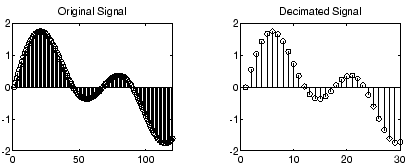
Figure 65. Illustration of a decimation filter
Low pass filtering is important in the decimation process to ensure no aliasing occurs. Aliasing refers to the effect of under sampling a high frequency signal and misrepresenting the high frequency behavior by a lower frequency. When aliasing occurs, there is no way to distinguish the erroneous aliased signal from the actual signal. The DSA hardware provides a decimation filter that uses a fixed proprietary low pass FIR filter with excellent ripple performance in the pass-band and very high attenuation in the stop band.
The decimation filter module contains multiple stages of decimation filters in the DSA hardware. (Figure 66) The data is decimated by a factor of two in each stage. After N stages of decimation, the data will be reduced to its 1/2N . The example provided in Figure 66 shows the decimation stage is set to 3 so the data will be reduced to 1/2^3 = 1/8 of its input points after this decimation module.

Figure 66. Decimation filter in the EDM software
The decimation filter is widely used to view, analyze, and record low frequency signals. For example, a system may be used to simultaneously acquire vibration and pressure or temperature data. While the signals are all sampled at a high data rate, the pressure channel and the temperate channel should be viewed and recorded at a much lower rate because these types of signals typically do not change dynamically (at a high frequency). In this case, users can simply apply decimation filters to the channels that measure and record pressure or temperature.
Integrating a decimation filter with other filter techniques allows the user to simultaneously analyze high frequency and lower frequency signals with different frequency resolutions. This capability is unique to the DSA system.
For example, users can apply a decimation filter to channel 1 in a CSA file as shown in Figure 67. This is an example from an application developed by Cystal Instruments.
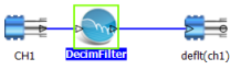
Figure 67. Decimation filter example
If a signal source with 1 kHz sine output is connected to channel 1 and the sampling rate is set to 64 kHz, the broad spectrum can be viewed up to 28 kHz as shown in Figure 68.

Figure 68. The auto spectrum of an 1 kHz sine wave when sampled at 64 kHz
However, users can also simultaneously display the spectrum of the decimated signal, decimated(ch1), with 8 times the frequency resolution as shown in Figure 69. Note that in this example the two spectra are of the exact same time signal, not of two samples acquired at different times.

Figure 69. The same sine wave at 1 kHz, after decimated 8:1, shows at different locations on the spectrum
A histogram is a graphical display that shows the number (or frequency) of events that fall into each of several or many specified categories. Figure 70 shows a typical histogram.

Figure 70. Typical histogram
Mathematically, a histogram is a mapping mi that counts the number of observations that fall into various disjoint categories (known as bins). Thus, if n is the total number of observations and k is the total number of bins, the total number of events is found by adding the frequency in all the bins as:

Cumulative Histogram
A cumulative histogram is a mapping that counts the cumulative number of observations in all of the bins up to the specified bin. That is, the cumulative histogram Mi of a histogram mi is defined as:

In DSA implementation, the Histogram and Statistics function is a single CSA module that can be applied to any time stream. The output of the Histogram and Statistics module is a histogram signal and the associated statistics results. Users can change the display format on the DSA.

Figure 71. Histogram example
A Crystal Instruments DSA provides the following measurement parameters for a histogram: bin number for the bar chart and amplitude ranges. It provides the following display formats for the histogram graph: normalized-linear, normalized-logarithmic, un-normalized, and cumulative. While the histogram is measured, it also provides the following statistics values: mean, max, min, RMS, variance, skewness, crest factor and kurtosis. The definitions of these statistics measures for N samples are:

The rms(x) is equal to the standard deviation when the mean is 0.
Skewness measures the asymmetry of data around the sample mean. If the skewness is negative, the data is spread out more to the left of the mean than to the right. If the skewness is positive, the data is spread out more to the right. The skewness of the normal distribution (or a perfectly symmetric distribution) is zero.
Kurtosis measures how outlier-prone a distribution is. The kurtosis of the normal Gaussian distribution is 3. Distributions that are more outlier-prone than the normal distribution have kurtosis greater than 3; distributions that are less outlier-prone have kurtosis less than 3.

As an example, a histogram of a Gaussian random noise is displayed in Figure 72.

Figure 72. Histogram of a Gaussian distributed random signal
Its cumulative histogram is displayed in Figure 73.

Figure 73. Cumulative Histogram of random Gaussian signal
Probability Density Function
An alternative view of distribution in a signal is the Probability Density Function. This is obtained by dividing the normalized values of a histogram by its bin width. Bin width is the difference between two consecutive values on the x-axis. The values on the x-axis are typical of the parameters being measured by the DSA.
The advantages of using a Probability Density Function are scaling of axis or preventing the change in histogram heights due to a change in bin width. The area under the Probability Density Function is always one.
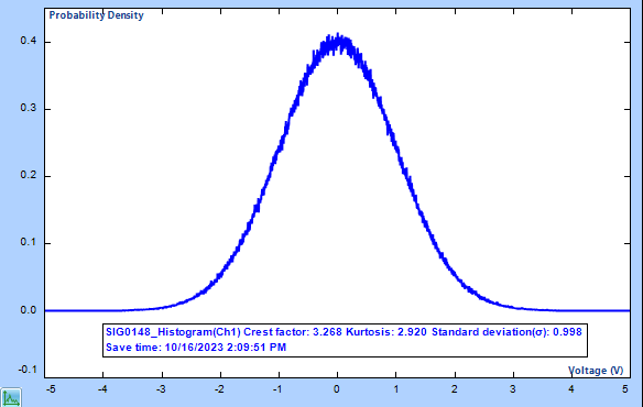
Figure 74. Probability Density curve of a drive signal