
Modal Analysis On Strut Parts
Download PDF | © Copyright Crystal Instruments 2016, All Rights Reserved.
Modal analysis is used to analyze the dynamic characteristics of structures and mechanical parts. This analysis, which identifies mode shapes and frequency and damping parameters, describes how the part reacts to dynamic forces. It is used for model verification, for assessing safety and performance, and for predicting the effect of design changes. Here, a CoCo signal analyzer, with ME’Scope software, is used for a modal analysis on an automotive suspension mount.
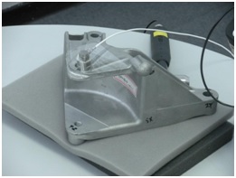
Figure 1: Automobile strut part
Test Conditions
The modal analysis procedure consists of numbering measurement points, establishing a geometric model, acquiring excitation and response signals, analyzing the signals, and determining the modal shapes and modal parameters. The data analysis involves applying data windows to the time streams, performing an FFT, and computing the APS, CPS, and FRF functions. The mode shapes are measured from the spatial variation of the FRF functions across the measure-ment points.
Modal analysis requires a data acquisition system and modal analysis post-processing software. In this case, we use Crystal Instruments’ CoCo-80 and ME’Scope, the modal analysis software by Vibrant Technologies.
The CoCo’s portability, accuracy, and high dynamic range make it well suited for modal analysis. It has a built-in IEPE current source for the accelerometers. It can do the data windowing and averaging and calculates APS, CPS, and FRF functions. It also has a Modal Analysis module that tags data with spatial coordinates which are imported directly in ME’Scope.
Test Settings and Steps
The part that will be tested is shown in figure 1. This part is from an automobile chassis of PATAC Co., Ltd. The structure of this part is quite complex and not amenable to analytical solutions.
The part was placed on a foam pad to simulate free boundary conditions. An instrumented hammer was used for excitation, and a single accelerometer measured the response. The response measurement point was fixed while several locations were used for excitation by the hammer.
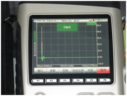
Figure 2: Time Domain Block Signal
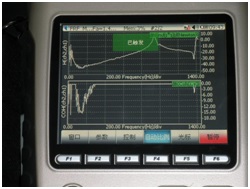
Figure 3: H and COH functions
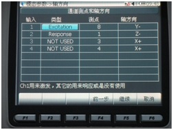
Figure 4: Excitation and Response Settings
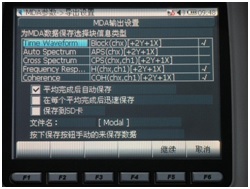
Figure 5. Modal Data Save Settings
In this experiment, we set analysis frequency as 2.56 kHz, average number as 4, with an exponential data window and the manual-armed trigger. No input range settings are required with the CoCo. With every hit of the hammer, the CoCo was triggered by the force transducer on the tip of the hammer. We then get time domain waveform and FRF data as shown in figures 2 and 3. This data is valid only if there is only one hammer hit per data block, which is visible in the excitation time signal, and if the coherence is near 1 which indicates a good signal-to-noise ratio. The CoCo operator can accept or reject the data frames with each hit of the hammer based on these criteria. In this case, since the average number was set to 4, four valid data frames will need to be acquired for every excitation point.
Before starting the test, the Signal Save Settings have to be set up as shown in figure 5. The Time Waveform, Frequency Response, and Coherence signals are selected to be saved. This data will be automatically saved to the CoCo’s SD card each time the average number is reached.
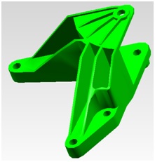
Figure 6. Pro/E 3D model

Figure 7. Excitation point locations and directions
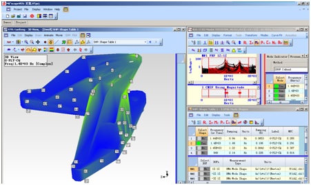
Figure 8. Modal data display window in ME’Scope
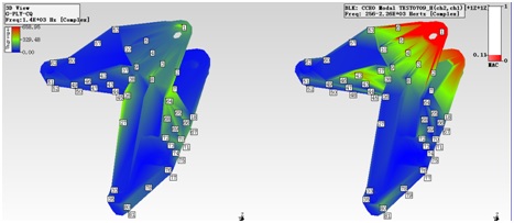
Figure 10. ME’Scope display of modes
For parts with complex geometry, it can become difficult to accurately enter the coordinates of all the modal points. ME’Scope simplifies this by directly importing the shape from CAD software such as Pro/E (figure 6). It can then apply the measurement points directly to the geometric model (figure 7). This makes it easy to efficiently and accurately generate models.
In addition, the shape also makes it difficult to describe the measurement axes in the form of X-Y-Z coordinates. In the ME’Scope model shown in figure 7, all measurement points are set in the Z-direction. ME’Scope can then set the Z axis of all points as normal to the surface of the part.
In EDM, or Engineering Data Management, is the desktop software used by the CoCo. After downloading the data from the CoCo, EDM can convert the FRF data to UFF format which can be opened in ME’Scope.
Since the CoCo tags each data point with coordinates, the FRF data is automatically imported to the correct point on the shape model. ME’Scope analyzes the resonant frequencies and damping factors of all this data to generate the modal shapes. All these modes can then be viewed and animated as shown in figure 9.
These modal parameters can then be used for model verification, structural dynamics simulation, FEA modeling, and design modification.
Conclusion
The CoCo and ME’Scope work well together to do accurate and reliable modal analysis. The portability of the CoCo and the simple user interface of ME’Scope minimize the set-up time. The ability to calculate mode shapes and modal parameters is a powerful engineering tool for analysis and design.