
The Modern Maturation of Machinery Monitoring
Download PDF | © Copyright Crystal Instruments 2016, All Rights Reserved.
Authors: James Zhuge, Ph.D. - Crystal Instruments, Santa Clara, CA | George Fox Lang, Hatfield, Pennsylvania
Invention and innovation characterize American life, but manufacturing sustains it. Smooth-running process machinery buoys and maintains the nation’s economy. Continuously monitoring the operating health and rapidly diagnosing the occasional mechanical woes of our nation’s production machines is a vital survival mission in today’s competitive business world. It is best accomplished by spatially distributed, yet tightly integrated, systems that bring measured questions from around the enterprise to any desired single point of analytic excellence for rapid operating decisions and informed run/repair choices.
The 19th century was a modern iron age, blessing us with all sorts of manufacturing machines and a variety of prime movers to drive them. Normal machinery maintenance was performed at regular service intervals as specified by the equipment manufacturer. Initial machinery monitoring was conducted by the operators using eye, ear and hand to sense process failure, unusual sound, excessive vibration or elevated temperature. This didn’t change much until the mid-20th century when electronic transducers and measurement instruments provided better ways to sense the health of process machinery. The screwdriver handle came off the occipital, and machinery dynamics were “listened to” using accelerometers, pressure gages and eddy-current proximity probes. As the century progressed, ingenious new displays better conveyed mechanical health to the human. These included narrow-band spectra, orbit diagrams, order tracks and waterfalls.
In the 1950-80 timeframe, analytic instruments moved into the field. Skilled analysts brought tuned filters and oscilloscopes, then time-compression spectrum analyzers, then FFT instruments to the machinery and gathered periodic operating “signatures.” Over time, the ability to detect abnormal signatures from machines developing mechanical faults and flaws was evolved. It proved possible to detect a broad range of developing machine degradations earlier and more consistently using these electronically aided senses. But the burden of lugging laboratory instruments to the field was onerous, and temporarily attaching sensors to the machinery was time consuming and sometimes inconsistent. Using knowledgeable machinery/measurement experts in a routed field-monitoring role was expensive. Substituting less skilled personnel often proved far more expensive.
Monitoring technology divided to follow two different strategic paths. Expensive plants and critical machines already had permanently installed sensors for process control. In more foresighted organizations, these were augmented by additional sensors added to monitor shaft-to-casing gap, bearing housing acceleration, bearing temperature and motor current. Like the process signals, these machinery health indicators were wired to the processing unit control room to be monitored by dedicated meters and indicators and to provide a plant-central point where more sophisticated analyzers could be occasionally attached.
Less critical machines (or those owned by the underfunded) were protected by routed measurements, now made using dedicated collectors and hand-held analyzers and a combination of man-carried and permanently installed sensors. These hand-carried instruments grew in capability and sophistication. Not only did their signal processing capability increase, these instruments also spawned dedicated data-base programs to plan and prompt routed measurement and to automate machine fault identification by comparing measurements against a library of previously identified faults.
Today’s Confluence of Concepts
Bringing measured machinery questions to the local unit control room is no longer sufficient. In the 21st century, information can be brought from any remote monitoring site to any location of technical competence. At such concentration points, measured results can be compared with operating experience of similar machinery at other locations. Tentative opinions may be experimentally examined by downloading new measurement instructions to the remote monitoring hardware. Trusted corporate experts (and their selected expert consultants around the world) can view measured data from any enterprise asset via the Internet using a personal computer, data tablet or smart phone. In short, time and global distance have been taken out of the diagnostic equation by modern network-capable equipment.
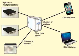
Figure 1. Crystal Instruments’ Spider-80X monitors and experts joined by a local-area network (LAN).
At most facilities, this is made possible by an Ethernet “backbone,” linking all processing units into a plant-wide LAN (Figure 1). At each processing unit, permanently installed monitoring transducers are wired to monitors at a sheltered proximate central point (typically a local control room). In turn, each monitor is connected to the Ethernet LAN. This allows the data to be viewed and analyzed anywhere the LAN has a port. An engineering data management (EDM) server program running on the LAN’s server manages data transfers to any computer on the network running the appropriate viewing/control software (client browser). Add an Internet modem to the LAN to provide a remote communication path to any computer in the world with Internet access. (Unplug that modem to isolate your LAN for maximum security if cyber attacks are a concern.)

Figure 2. Crystal Instruments’ Spider-80X monitors and experts joined by the Internet.
At facilities lacking a plant-wide Ethernet backbone, the Internet may be used as a substitute path, as shown in Figure 2. Any combination of broadband telephone, cable or wireless connection to the Internet is fair game. A cellular modem connected to a monitor provides a true stand-alone measurement subsystem. While line power is almost always available within a processing plant, it may not be for other applications. Monitoring bridges, wind-powered generators, road profiles, flutter testing or airport noise may call for a battery-powered installation, perhaps one with solar (or other) backup. For this reason, the monitoring hardware should be fully capable of running (at full performance specification) from low voltage DC as well as domestic, overseas and aircraft AC line power.
Every measurement sub-system must collect and transmit only the highest quality data. Measurements must reflect the highest fidelity possible. They must be precise and resolute in every dimension including time, frequency and amplitude. This means available sample rates must be high enough to capture the most rapid transient event. Additionally, it must be possible to synchronize sampling of modules separated from one another. This implies use of IEEE 1588v2 Ethernet communication protocol. It must also be possible to record and retain long time histories to facilitate post-computation of resolute spectra. This implies deep memory in each monitoring module.
Finally, the amplitude measured in any domain must exhibit high dynamic range to detect quiet problems in the presence of a loud background. The measurement instrument must have superior analog input circuits, the finest analog-to-digital converters available and the facility to convert measured time histories to floating-point format before anything else is done with the data.
A Bit About Bits and Converters
There are many ways to build an analog-to-digital converter (ADC). One type of converter, called a successive approximation converter, dominated audio frequency spectrum analysis since the first time-compression, real-time analyzer (RTA) appeared in 1957. The successive approximation converter offered several benefits for instrument applications, including rapid conversion (i.e., high sample rate), compatibility with an input multiplexer (a cost savings for multi-channel analysis at lower frequency) and the ability to use a variable sample rate (then necessary to produce an order-normalized spectrum).
These components were initially hand-filling potted modules of 8-10-bit precision accepting sample rates in the hundreds of kHz. As silicon sculpturing matured, the successive approximation ADC shrunk to a chip and grew to 16-bit precision with sample rates as high as 4 MHz. While these ADCs have become cheaper, smaller and faster, they have not become more resolute. The successive approximation converter’s resolution is limited by the need to use very precise resistor values within its circuitry. Errors in the resistor values produce uneven bit steps with voltage changes, very undesirable for spectrum analysis, since they cause harmonic distortion.
Cellular telephony gave rise to a very different type of ADC, the delta sigma (DS) converter. In this type of converter, the analog signal is first very coarsely quantized by a one-bit serial converter at a very high sample rate. The resulting serial bit stream is played through a digital reconstruction filter whose parallel output is sampled at a much lower sample rate.
The design of the digital filter and the ratio of input and output sample rates determine the number of output bits. DS converters were originally thought inappropriate for use in mechanical equipment analyzers, because their sample rate needed to be constant and the input could not be multiplexed. However, these parts rapidly grew to 24-bit precision and dropped dramatically in price. They also demonstrated another major benefit: they did not require a complex analog anti-aliasing filter – eliminating a lot of components, reducing cost and saving precious printed circuit acreage. It became economically feasible to use one DS converter per channel, even in inexpensive instruments. The variable sample rate obstacle was overcome with the development of digital re-sampling order analysis. This algorithm eliminated the need for an external phase-locked loop/voltage-tuned filter tracking adaptor previously required to produce an order-normalized spectrum.
Spectrum analyzer designers love DS converters because they exhibit far lower differential nonlinearity (DNL) and integral nonlinearity (INL) than successive approximation ADCs. Converters with low DNL have a very consistent voltage step between bit-adjacent output codes. Those with low INL have a very linear volt/step transfer function over the entire code range. These characteristics result from the 1-bit quantization performed by the delta modulator, and they produce clean spectra with low harmonic distortion. So, 24-bit DS front ends have become the standard of the audio frequency analyzer industry. This is unlikely to change in the next few years. While several chip manufacturers now offer 32-bit parts, they only operate at low output sampling rates (4 kHz typical), and this barrier is going to take some time to overcome. So here in 2014, a 24-bit front end sets the standard for analyzer dynamic range. Or does it?
Automating Headroom
Headroom is the amount of gain you must give up in a recording session to assure that the result will not be clipped (overloaded). Twenty-four-bit resolution is quite adequate for virtually any analysis in the time, frequency, order or amplitude domains – but only if the channel sensitivity is properly matched to the signal. An overloaded channel conveys little information other than that the signal is too large to be properly understood. An important signal buried in the noise floor of an insensitive channel is equally uninformative. This is not a new problem; it is one that begs for a solution in many industries. U.S. Patent number 7,302,354 may provide that answer.
Consider the challenge of recording a band in concert. Some of the songs will be quiet, while some will be loud. How do you set your recording levels? A friend who does this professionally shared his recipe – ask the band to give you a sample of their loudest number first, and then set the required gains as 0 dB on your board. Be prepared to “ride the board” during quieter tracks, providing more gain to those musicians (channels) that need to be heard during a quiet number. This is a difficult algorithm to emulate in machinery monitoring. You cannot ask a machine to provide its loudest signatures during setup. You may have some opportunity to have the operator vary process load or other parameters, but don’t plan on the monitored “band” giving you either its most exuberant or restrained performance on demand.
Laboratory instruments have always been well served by input attenuator knobs used to select each channel’s full-scale sensitivity. However there is no one watching a remote monitor to make such an adjustment. On the surface, some form of auto-ranging might seem to answer this problem. However, that’s not really true. If you are monitoring and the signal level changes enough to require a range change, you’re going to miss recording or analyzing exactly that event you want to capture and understand while the system re-determines the proper measurement sensitivity. If the event is a transient increase, by the time you come “out of the blind” it will be over, and the channel gain just selected will now be too low. Clearly, neither knobs nor auto-ranging provide the right answer in a remote monitor! In fact, the ideal unattended monitor input channel has a fixed full scale slightly greater than the largest signal the transducer feeding it can produce. This must be accompanied by sufficient channel dynamic range to clearly measure the smallest meaningful signal the transducer can generate. A 24-bit ADC provides output integers spanning 144 dB (a 1.6 million to 1 ratio). However, the actual measurement channel will never produce this great a dynamic range.
The actual ratio of smallest-to-largest voltage that may be simultaneously detected is better described by the converter’s effective number of bits (ENOB) measured per IEEE Std. 1241-2000. Properly applied to today’s 24-bit converters, this is in the 18-20 bit range, yielding a 108-120 dB dynamic range. For a practical full-scale value of ±20 volts, this means signals in the 20-80 μV range can be reliably detected. But U.S. Patent number 7,302,354 provides a means of opening the usable dynamic range to 150 dB, allowing signals as small as 600 nV to be detected.
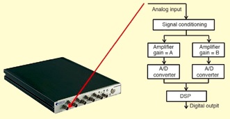
Figure 3. Hardware per U.S. Patent 7,302,354 applies two ADCs and a DSP to each input channel.
How is this accomplished? As shown in Figure 3, by applying two ADCs and a digital signal processor (DSP) to each measurement channel. The analog circuitry preceding each ADC is identical, except the amplifier voltage gains differ by a factor of 100. So if the low-gain path (say A) has a full-scale range of ±20 V; the highgain path B has a full-scale of approximately ±200 mV. During a measurement, both converters run all the time, and their digital output streams go to a DSP which implements the patent-protected “stitching” algorithm that seamlessly blends the two sample sets.
During most operations, the B path is overloaded, and its data are without value. But when the signal strength diminishes, the fact that the B data is no longer overloaded can be ascertained from the high-order bits of the A data stream. The output then switches over to use the amplified results that give far better fidelity at low amplitude. Should signal strength again increase to clip the amplified path, this is detected from the unamplified data, and output focus shifts to the low-gain path.
During intervals where both A and B data paths are known to be in band, the DSP implements a cross-path calibration curvefitting procedure, whose results virtually eliminate any distortion at the cross-over points between the two signal paths. Therefore, the continuously available dynamic range of the channel is significantly increased by better than 30 dB. To achieve this high level of performance, the hardware must be optimized for close phase match between the high and low gain paths. To this end, the two ADCs share a common silicon substrate as well as power supplies and sample clock.
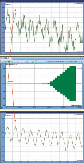
Figure 4. Comparison of A and B path measurements at low amplitude show superiority of high-gain data.
The upper and lower expansions in Figure 4 illustrate the superiority of the B path data at low signal amplitude. Most of the middle measurement (stitched from A and B data) display is dominated by the low-gain A path, while the B path is in overload. The enlargements compare the competing A and B path data streams in a low amplitude region prior to stitching. Clearly the high-gain B data are cleaner and far more resolute in this region.
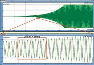
Figure 5. Magnified view of stitched data shows continuity across multiple A-to-B and B-to-A transitions.
Figure 5 demonstrates the success of cross-path calibration. The lower expansion illustrates multiple crossings between the A and B gain paths. The measurement is smooth and continuous with no sign of a glitch at any of these transitions.
The cross-path calibration is actually applied to every sample at the same time it is being converted to physical units in floating point format. The resulting time history is retained in a stream of 32-bit, single-precision, floating-point words (per IEEE 754-2008). This format retains a sign bit, 23 fraction bits and eight exponent bits in four bytes. Values between ±1.8 ¥ 10–38 and ±3.4 ¥ 1038 can be represented with better than seven-digit precision. Restated, the floating-point format provides 140 dB precision anywhere within a 1525-dB numeric range.
Why Emphasize Dynamic Range?
Machinery monitoring can be a bit like the definition of flying an airplane – hours of boredom interspaced by seconds of sheer terror. In those few anxious seconds, well-guided decisions are all important. Your continuous monitoring system must really be continuous to fully protect your equipment. A momentary blip on the monitoring radar may convey a strong hint of unsavory events that might occur with a change in process settings. For example, evidence of a momentary shaft rub will lead the astute operating team to assure all bearings are receiving clean oil at the proper pressure before changing the system speed.
Anytime a new (or refurbished) process train is started, valuable information about the correctness of its assembly is exhibited in the rapidly changing proximeter, accelerometer, current transformer and pressure sensor signals. This is the time to watch all signals closely; it is not the time to be adjusting input channel gains! Further, during a startup you might need to study a relatively large (and slowly changing) DC value accompanying a small AC signal –as in tracking a shaft center-line position and associated dynamic shaft orbit. You want both diagnostic cross-plots to have the best possible amplitude fidelity; this calls for as much dynamic range as you can provide to view and analyze both of these informative but infrequently available shaft-to-casing gap signatures.
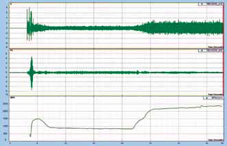
Figure 6. A machine in transition (typical start-idle-accelerate-run cycle shown) can exhibit high-amplitude transients.
Conclusions
While many steady-state operating problems are identified by near-DC measurements, such as temperature, oil quality, lubricant debris, shaft axial position and bearing journal oil pressure, dynamic measurements made during speed or load variation can offer unique insight into a machinery train’s health. A typical machine run cycle is shown in Figure 6. An anomaly detected during a routine process change can alert the need for more detailed dynamic measurements (and their storage) at the next operating perturbation. Every commissioning startup and end-of-turn shutdown should be documented with measurements of shaft orbits, shaft centerline positions, and waterfall displays.
Eliminating the need to adjust any channel’s sensitivity is an important contribution to truly continuous monitoring. But, today’s modern monitoring systems facilitate agile operation as well as dealing with agile signals. They can be rapidly reconfigured from afar to change from routine monitoring measurements to those required to document a shutdown or restart or analyze an anomaly. Modern software provides all of the necessary facilities (and security safeguards) to achieve such flexible operation without being distracted from the basic monitoring mission.
Modern purpose-built measurement hardware takes full advantage of today’s communication networks to provide continuous monitoring and superior diagnosis of process equipment. These modern solutions permit more machines distributed in more corners of the globe to be more carefully operated and maintained by fewer people working under less stress. Day-to-day marvels such as cellular telephony and clouds of Internet data storage facilitate this economic wonder. But to capitalize on these gifts, cost-effective monitoring systems need to incorporate new measurement components designed from their conception to function in this new communication environment.
The Crystal Instruments Spider System
The heart of the Crystal Instruments monitoring system is the Spider-80X module, a tiny (239 ¥ 216 ¥ 20 mm, 1.3 kg) signal processing powerhouse monitoring eight analog signals and two tachometers. Each analog input is serviced by two, 24-bit ADCs and a DSP implementing the cross-path calibration technology of U.S. Patent number 7,302,354 B2 to achieve better than 160 dBFS dynamic range (simultaneously measuring signals as small as 600 nV and as large as ±20 V). Some 54 sample rates from 0.48 Hz to 102.4 kHz are provided with better than 150 dB of alias free data from DC to 45% of any selected sample rate protected by steep 160 dB/octave anti-aliasing filters. The eight channels are amplitude matched within 0.1 dB and phase matched within 1°. The tachometer channels accept pulse trains of 3-300,000 RPM (0.05 Hz-5 kHz); these are sampled with 24-bit resolution.
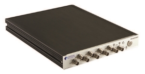
Spider-80X module accepts eight analog signals and two tachometer signals through front panel BNC connectors; it provides a power switch and status LEDs (power, run/stop, flash memory capacity, LAN communication).
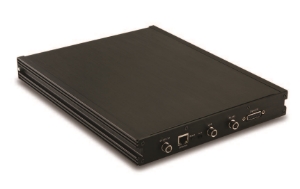
Rear panel provides a 100Base-T female RJ45 Ethernet connection, a LIMO five-pin Spider-NAS port, an RS-485 serial port, a DB25 Digital I/O connector and a 15 VDC (±10 %, 10 watt) power input connector.
The Spider-80X links to a local computer, LAN or the Internet via Ethernet. Measurement instructions are uploaded to it and data are retrieved from it. Dedicated digital I/O and RS-485 serial connectors are also provided for custom system integration. Each Spider-80X module contains a 4-gigabyte flash memory. This memory may be used for any combination of processing instructions and data storage. If additional memory is required, a dedicated interface is provided to exchange data (at 819,200 samples/second) with a Spider-NAS module. Spider-80X requires 10 watts of 15-VDC power drawn from an external supply. A single Spider-80X module can serve as a complete networked monitor.
The Spider-NAS (network attached storage) module provides 250 GB of solid state disk (SSD ) storage in a removable SATA cartridge. One Spider-NAS can record streamed time waveforms and spectra from up to eight Spider-80X modules.
Multiple Spider-80X and Spider-NAS modules may be ganged together using a Spider-HUB. In addition to facilitating Ethernet communication between the modules and a networked controller, a Spider-HUB forces sample synchronization across the interfaced modules. Time-stamping accuracy is better than 50 nanoseconds though use of IEEE 1588v2 technology. Alternatively, the fan-cooled S-80X-A35 mainframe is available to house up to eight Spider-80X modules. This rugged chassis provides both the Spider-HUB and Spider-NAS capabilities prewired to the modules and provides power.
References
Zhuge, James, “Cross Path Calibration for Data Acquisition Using Multiple Digitizing Paths,” U.S. Patent number 7,302,354, November 27, 2007.
Anderson, Ole Thorhauge, and Jacobsen, Niels-Jorgen, “New Technology Increases the Dynamic Ranges of Data Acquisition Systems Based on 24-bit Technology,” Sound & Vibration magazine, April 2005.
Lang, George Fox, “Quantization Noise in A/D Converters and National Elections,” Sound & Vibration magazine, November 2000.
Deery, Joe, “The Real History of Real-Time Spectrum Analyzers,” Sound & Vibration magazine, January 2007.