
Spectral Processing for Time Stamped Signals: Theory, Implementation, and Application Examples
Download PDF | James Zhuge, Ph.D. - Chief Executive Officer
© Copyright Crystal Instruments 2023, All Rights Reserved.

Abstract
CI recently released an accurate time stamping technology that uses GPS as a time source. The technology is deployed on the CoCo-80X portable analyzer and GRS, CI’s latest product for acoustic applications.
The time marks can be as accurate as 100 nanoseconds. Using this time stamping technology, we developed the theory and algorithms to calculate the auto and cross spectrum between measurement channels on separate data acquisition units that can be distanced thousands of miles apart.
Other traditional time sources, such as IRIG-B, can be used in the same manner as a GPS time source. In this paper, we mainly address the technical issues raised in using a GPS time source since it is a new technology in our industry.
Traditionally, measuring the transfer function between any two sensors requires that all ADC (Analog to Digital Converters) are accurately synchronized through a hardware connection. Synchronizing the sampling clocks of all ADCs is accomplished when all the data acquisition units are located nearby. Crystal Instruments has developed Ethernet based time synchronization technology that can extend the cable length up to 300 feet. The ADC clock synchronization will become difficult and unreliable beyond 300 feet. The technology presented in this paper provides an alternative approach. Instead of synchronizing the ADC sampling clocks, this new technique only requires accurate time stamping to the sampled data points.
This technique allows measurement channels that are separated by a large distance to synchronously acquire data without any connected wires.
In all typical FFT analyzers, the following spectra are always computed: auto power spectra of all measurement channels, cross-spectra of any pair of channels, transfer function (or FRF, the Frequency Response Function) of any pair of channels, coherence functions of any pair of channels, and phase spectra of any pair of channels. Once the auto power spectra and cross-spectrum of a pair of channels are computed, the other signals can be derived. Since the auto-power spectra computation is very simple and requires no cross-term information, the only question remaining is how to compute the cross-spectrum of any pair of channels that are from different GRS or CoCo units and are accurately time stamped.
Signals are received from separate GRS or CoCo units, so a new algorithm was developed to correct the phase mismatch between any pair of FFT spectra based on certain calculations of time stamps. Typical tests indicate that the GRS or CoCo can achieve the following specification for the phase estimation of the cross-spectral calculation:
| Phase match between two GRS or CoCo units: |
±2°(degree) at 40 kHz ±1°(degree) at 20 kHz ±0.5°(degree) at 2 kHz |
This is an extraordinary result. While many companies claim to use a GPS time base for their data acquisition, we have not observed any other companies claiming to achieve such an outstanding cross-term spectral analysis performance.
This accurate time stamping technology can also be used indoors. CI performed a test using the GPS repeater inside a commercial building. The performance of time stamping technology was as good as using it outdoors.
Potential Applications
This technology has many potential applications. Essentially, any structure or acoustic measurement that requires multiple sensors distributed across a large distance can now use the GRS/CoCo to perform the measurement. After obtaining the measurement, the cross-channel terms can be calculated with greater accuracy.
1. Sound Boom Measurement for Aircraft
The contract awarded to CI by NASA intends to use hundreds of GRS units spread across 10,000 square miles to simultaneously take measurements. While the contract did not specify the details of the time stamped signal processing method described in this document, the technology can certainly be used to analyze the sound boom effect with much higher time accuracy.
2. Measure the vibration mode of large bridge
Using only two GRS units and by roving the measurement points, it is possible to measure the operating deflection shape of a very large bridge. All we need is a sequence of FRF measurements in pairs.
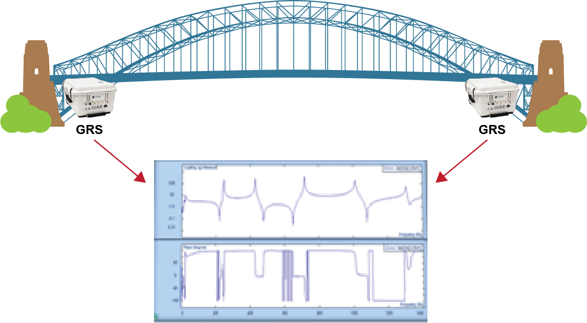
Figure 1. Compute the frequency response, phase, cross spectrum, or coherence functions between two distant points
3. Vibration mode of large vehicles
The GRS or CoCo is ideal for measuring the vibration mode of ships, aircraft, large trucks, bullet trains, railways, large cranes, and other large structures.
In theory, two GRS or CoCo units can acquire data across the earth’s diameter, and we can calculate the transfer function between the measurements of these two systems. But we have not seen a need for it.
The only limitation of this technology is that the data acquisition systems need to receive GPS signals. Without GPS signals, the time stamps are not available.
4. Any indoor application that requires time synchronization
GPS repeaters can be used to redistribute the GPS signals inside of buildings. This method allows the user to replace all previous wired high channel data acquisition systems with multiple unwired GRS or CoCo-80X units. The major advantage of doing so is to drastically reduce the wires between the measurement instruments. The data acquisition front-ends can be positioned closer to the clusters of sensors instead of using very long cables.
Analysis of GPS Time Stamps
Technology background of time stamping
The Global Navigation Satellite System (GNSS) installed in the GRS or CoCo delivers high integrity, precision timing for demanding applications across the world. Support for BeiDou, GLONASS and Galileo constellations - in addition to GPS (Global Position System) - enables compliance with national requirements. Enhanced sensitivity and concurrent constellation reception extends coverage and integrity to challenging signal environments. Survey-in and fixed-position navigation reduce timing jitter, even at low signal levels, and enable synchronization to be maintained with as few as one single satellite in view.
Due to the popular use of the term GPS (Global Position System) in history, this document simply adopts the usage of GPS instead of GNSS.
In a data acquisition system where the time accuracy of the sampling clock is not very demanding, say no better than seconds, the time base can be derived from the “computer time”. This can be set manually, through a time server on a network, or through the internet. When the time accuracy of the sampling clock demands millisecond resolution, the digital input paths of the data acquisition system - especially its ADC - has to be designed with control from a more accurate time base, such as GPS or IEEE 1588 PTP (precision time protocol). This is necessary to calculate the cross-channel spectrum, or any signal property related to the time delays between all measurement signals.
If the ADC sampling clocks cannot be accurately synchronized between different hardware units, it is possible to achieve similar signal processing results if all recorded data is accurately time stamped. Applying time stamps and synchronizing the ADC clocks are two different strategies. CI believes that with accurate time stamping, the users should be able to achieve the same measurement goals, including calculating the cross-spectra between all measurement channels.
Multiple GRS or CoCo data acquisition systems can acquire data at the same time while they are physically spread out over hundreds of miles. These units do not share any direct hardware connections except that each will receive GPS signals. Accurate time stamping technology is implemented with the GPS time base to allow the acquired signals to line up in Crystal Instruments’ post processing software, Post Analyzer (PA).

Figure 2. Outdoor application
The Global Positioning System, or GPS, consists of 24 satellites revolving around the earth every 12 hours. Each of these satellites has an atomic clock onboard with extremely good accuracy. The GPS satellites continuously transmit their coordinates in space along with a time message on a 1.575 GHz carrier frequency. The GPS receiver used in the GRS or CoCo claims to achieve ±60 ns time accuracy at 99% of time.
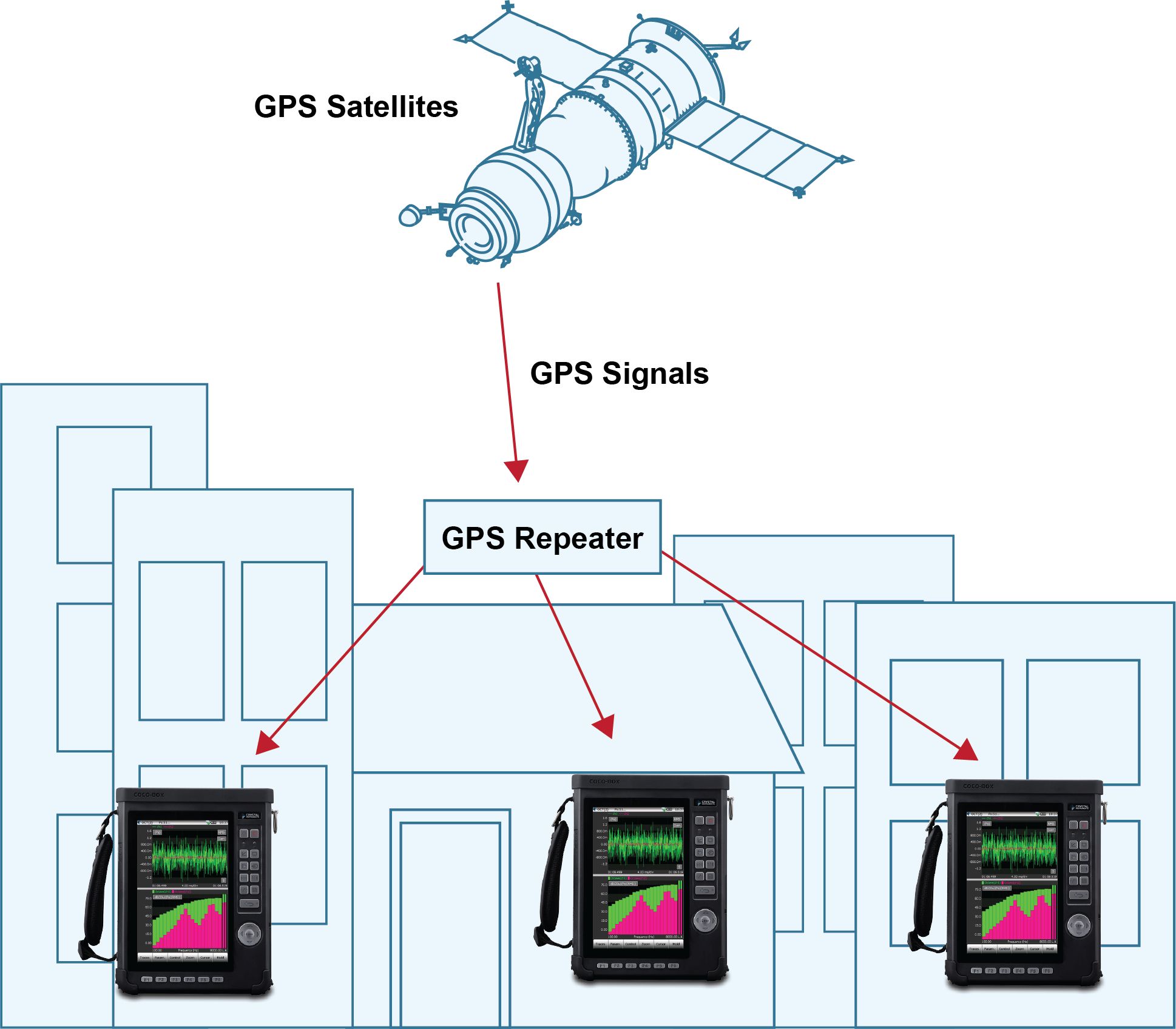
Figure 3. Indoor Application
For indoor applications, one of multiple GPS repeaters can be used to transmit the GPS signal and rebroadcast it inside of the building.
Clock Drift Analysis
Clock signals, timing and location signals can be derived from the GPS chip signals inside each GRS or CoCo unit. A real-time, zero latency hardware logic is implemented to time stamp the A/D sampling clock with the measured GPS time base.
A simplified diagram of how time stamping works in the GRS or CoCo is shown below:

Figure 4.
In the hardware, a time register is derived from the GPS receiver chip that is directly accessible by the FPGA and the processor. The GPS timing accuracy is better than ±60 ns with 99% probability according to the specifications of the GPS chipset. The time stamping method described above results in time stamping accuracy within the sub-microsecond range, typically less than 100 ns.
Given such an accurate technique of applying time stamps, we are able to analyze the error of actual sampling clocks vs. the GPS time base, which is described as follows.
An ADC requires a clock with a specific oscillator frequency to drive its sampling. The diagram below shows the ADC clock drift in concept. Here the ADC clock has a period of more than 10 μs (102.4 kHz ↔ 10 μs sampling). The drift might be caused by the environment, especially changes in temperature.
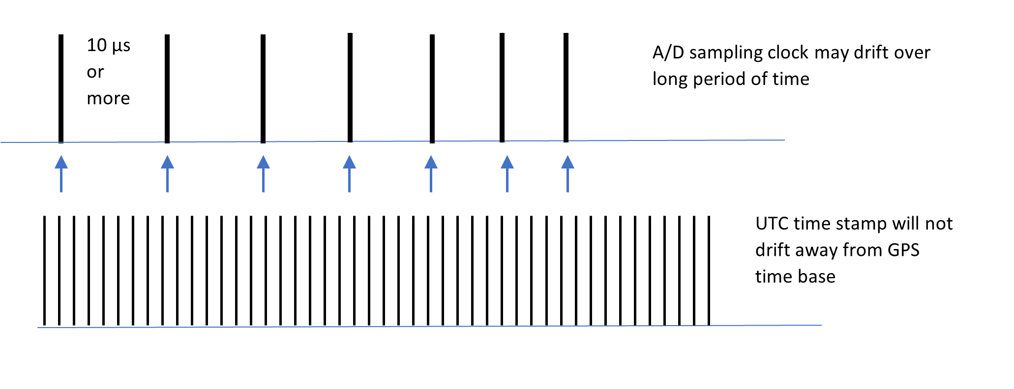
Figure 5.
Besides the short term drift, the ADC sampling clock - which is driven by an internal oscillator in the hardware - may have an inherent offset compared to oscillators on other GRS or CoCo units, or compared with the atomic clocks used by GPS time. The combination of offset and drift produces a bias of the clock. For a recording time of a few minutes this bias may not be a major problem. However, if the recording time is as long as hours or days, this sampling clock bias may cause sampled data from different units to have mismatches when comparing time stamps.
Bias error = short term drift + offset
Suppose the oscillator that drives the A/D sampling has a stability of 50 ppm (part per million). After one hour the clock bias will be the following:
(0.000050 bias) * (3600 seconds per hour) = 180 ms bias error per hour
In the worst case scenario, the time clock of sampled data will vary by a factor of 180 ms per hour. This situation occurs when all oscillators on different units are running without clock constraints, such as periodic synchronization through a GPS signal.
In order to discuss the timing issues with clarity, a few terms used in this document are introduced:
Nominal Sampling Rate is the sampling rate labeled by the product specifications, for example, 64 kHz, 102.4 kHz etc. They are not accurate because of the bias and drift of the ADC clocks.
Nominal Time is the time of acquired signal samples calculated based on a starting time, number of samples and nominal sampling rate.
Measured Time is a series of time stamps taken from the GPS clocks corresponding to the samples of acquired signals. If the GPS works properly, the Measured Time is a much better time base than Nominal Time.
Corrected Sampling Rate is a single value for the sampling rate used in the entire duration of a recording. It is calculated by removing the offset between local clocks against that of GPS based on the Nominal Sampling Rate, duration, and Time offset.
In other words, the Corrected Sampling Rate is calculated by removing the first order error between the local clocks and GPS time base.
The GRS/CoCo is able to record time stamps and display them in the following format:
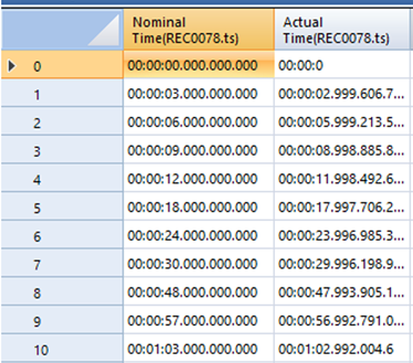
Figure 6.
When drawn in a plot using (Measured-Nominal) vs. Nominal, it will look similar to the following screenshot:
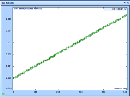
Figure 7.
In this example of roughly 500 seconds of measurement, the nominal time is off by 5 milliseconds against the GPS time clock. In this particular case, the local clock is slightly slower.
The 5 milliseconds error from 500 seconds of measurement is within the range of expected error of the oscillator. But it is too large to conduct signal processing when cross-channel computation is needed. For vibration and acoustic applications, the time base difference between the data samples of any two channels must be within a few microseconds of each other.
Since we know the error between nominal time and actual measured is mainly an offset instead of random drift, this offset error can be corrected after taking the measurement. The technology developed to create the GRS or CoCo first applies a correction to the sampling rate, then uses the signals with the corrected sampling rate in post processing. The following describes the correction process with more details:
1. Calculate the Time Offset as shown in the previous plot for the entire duration of the measured signals, 504 seconds in this example.
2. Based on the duration of measurement and the time difference between that of nominal and GPS time stamps, the actual measured sampling rate is calculated as:
Corrected Sampling Rate = Nominal sampling rate / (1.0 + Time Offset/Duration)
For example, if the Nominal Sampling Rate is 64 kHz, the Time Offset is 0.005 second and Duration is 504 seconds,
Corrected Sampling Rate = 64 kHz / (1.0 + 0.005/504.0) = 63.999365 kHz
3. This Corrected Sampling Rate is computed by removing the first order error from the nominal sampling rate. It did not take the sampling rate fluctuation into consideration during this time period.
4. Since we know the signals acquired on this unit come from a slower clock of 63.999365 kHz, we are able to adjust it in the display and post processing algorithm.
The following is an example of how the corrected sampling rate can help in data processing.
In the plot below, it shows that when an impulse event is recorded by two data acquisition systems with slightly deviated sampling clocks, the signals will be off by a certain duration even with the same starting time-base.

Figure 8.
But after a correction against the GPS time base, the sampled points can be lined up on the plot.
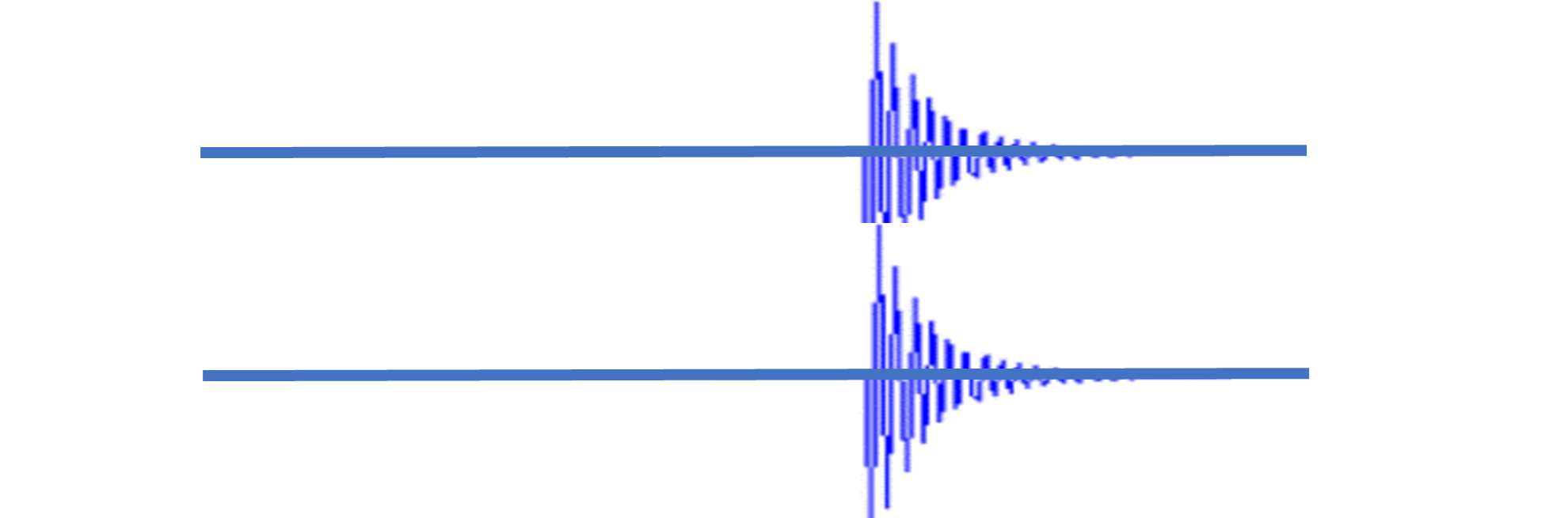
Figure 9.
After the adjustment, all classic signal processing methods such as FFT, FRF (Frequency Response Function), Coherence Function etc., can be applied using the post processing software.
The next question asks how accurate the Corrected Sampling Rate is. The post processing software is able to display the clock fluctuation after the first order correction. The following two graphs display the “drift” of the time stamps after the correction is applied.
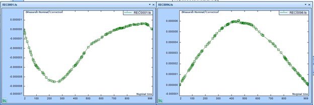
Figure 10.
Both vertical and horizontal are displayed in units of seconds. In these graphs, the quantity displayed vertically is:
(Measured – Nominal) – Correction
The Correction is a straight line drawn between the two time stamps, the very first and last time stamps of the entire recording. Both signals show that the fluctuation range is roughly 6 µs while the recording time is roughly 1000 seconds.
This fluctuation will be further corrected when a more sophisticated clock correction algorithm is used, which is already implemented in the Crystal Instruments PA software.
Calibrate the fixed offset of time stamps
The ADC and filtering processing chain in the GRS data acquisition system will introduce a fixed time bias to the time stamps. This time bias is governed by the sampling rate.
The following diagram shows the three areas that will contribute to this time bias error.

Figure 11.
ADC filter delay: the built-in FIR filter in the sigma-delta ADC has a certain delay effect. The time delay depends on the filter type that the hardware is initialized to, and the sampling rate. Since the filter type will never change on a unit, the only accessible parameter is the sampling rate. The ADC sampling rate is selectable from 8 kHz to 102.4 kHz in multiple stages. Each sampling rate setting will have a fixed amount of time delay for ADC.
FPGA temporary buffer (part of propagation delay): The time stamps are attached to the input sampled data in the FPGA. The FPGA may have certain temporary buffers that may cause a certain amount of time delay. The length of these temporary buffers is fixed. Therefore, the time delay caused by FPGA is also fixed.
Decimation filter on DSP (filter delay): at a sampling rate lower than 8 kHz, one or multiple FIR decimation filters will be inserted at the DSP level. The decimating filters will cause a fixed time offset bias. The only determining factor is the user selectable sampling rate.
In summary, given a sampling rate setting from the user interface, the time bias error is a fixed constant number across all hardware input channels. To correct this bias error, it is simply a matter of adding a correction table to all time stamps with the input parameter of a sampling rate. The recorded data will have time stamps with bias removed.
The signal plot example below shows how after the time offset bias is completely removed, the 1 pps (Pulse per Second) GPS signal is fed into one of the input channels.
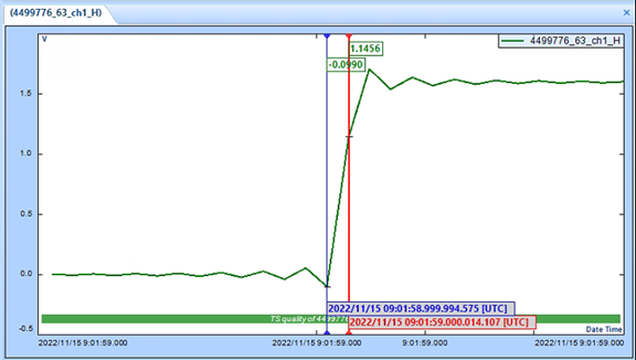
Figure 12.
The data is sampled at 51.2 kHz. The time interval between any two discrete points is about 20 µs. The two cursor values show the UTC time stamps at two discrete points. The timing of the rising edge of the 1 pps signal is from the GPS chip mounted on the board. It can be traced back to the National Institute of Standards and Technology (NIST) time source. The rising edge of the pulse shown in this example is at the following time:
2022/11/15 09:01:59 [UTC]
The time at the blue cursor is about 6 µs less than this “integer” seconds while the time at the red cursor is roughly 14 µs more than this “integer” seconds.
After the bias removal, the absolute value of time stamps will have no offset error.
Determining the interval of time stamps
In the GRS or CoCo system, the time stamp intervals are set as 5 seconds. A time stamp is taken roughly every 5 seconds. The time stamps and geographic location data values are saved into a separate file (.TS file). The file will be encrypted and saved into the SD cards.
The choice of 5 seconds as a time stamp interval is not arbitrary. We chose this length based on the following factors:
Considering the drift error of the local ADC clock is 10 ppm, we calculate the biggest possible time error of an ADC clock for a time stamp interval as larger than 5 seconds.
Using the cross-spectrum analysis method described below, we analyze the largest possible phase shift when increasing the interval of time stamps.
The interval should not be unnecessarily too small in order to save memory space.
It is found that if we increase the time interval of time stamps to beyond 100 seconds, the phase measurement using the cross spectral method will show an unacceptable deviation. But as long as the time interval of time stamps is less than 60 seconds, the phase measurement of cross spectrum is always good. Therefore, a 5 second interval is a very conservative choice.
When time stamps are lost during data acquisition
The GRS and CoCo have independent ADC clocks that drives the ADC sampling and a system clock that keeps the local time and calendar. When GPS signals are not available, the time stamps and geographic location information will not be available. But the data acquisition systems can still conduct normal data acquisition operations.
The GPS timing base, if available, will be assigned to the system clock each time the GRS is booted up. This means that the system clock will be frequently adjusted based on the GPS time base.
If the GPS signals are not available when the system is booted up and the data acquisition starts:
The GRS or CoCo system will assign its previously saved location coordinates to the ATFX file header.
The GRS or CoCo system will assign its system clock value, which is less accurate than that of GPS, to the ATFX file header as the starting time.
The .TS file will be filled with a mark of “****TS lost****” since time stamps are not available for use. A sample of a time stamp display with TS lost is shown below.

Figure 13.
If the GPS signals are not available during the initial stage of data acquisition, but returns during the operation:
The .TS file will be filled with a mark of “****TS lost****” in the duration that time stamps are not available to use.
When GPS signals are good, the system will start to record the location and time stamps into the .TS file
The GRS system will recalculate the acquisition starting time based on GPS information and save it to the ATFX file header.
Our experience indicates that if the GPS signals are lost for about 60 seconds or less, the quality of time stamps will not affect the measurement. But if the GPS signals are lost for longer than 100 seconds, the cross spectral analysis will not achieve good phase quality.
An example of time alignment
The following is an example demonstrating how the signals are plotted after a sampling rate correction is applied using attached time stamp signals.
Original file name: REC0058, REC0131. These are recorded on two GRS units. When they are recorded, a source signal is fed into the input ends of both units using a T-splitter port. Both GRS units have installed GPS receivers to communicate with GPS satellites. The recording duration is about 40 minutes.
Nominal sampling rate:
REC0058: 20,480 Hz
REC0131: 20,480 Hz
Sampling rate after the first order correction:
REC0058: 20,480.026214158832 Hz
REC0131: 20,480.011221929413 Hz
The following plot shows these two signals in the time zone of the triggering point:
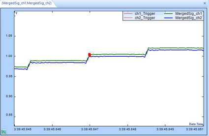
Figure 14.
The following plot shows the transient event at the end of a recording without a sampling rate correction. It shows the time difference between two signals is about as large as 36 sampling points:
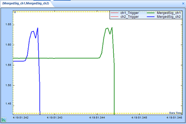
Figure 15.
The time difference shown above is caused by using the nominal sampling rate, which is inaccurate.
The following plot shows the same transient event at the end of a recording while the first order correction is applied to the sampling rate of both signals:
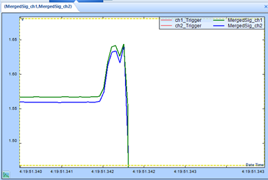
Figure 16.
The two signals are lined up beautifully on the horizontal axis.
Spectral Analysis based on Time Stamped Signals
Summary
With recorded signals gathered from multiple units, the processing algorithm is summarized in the following steps:
First, the user will need to enter typical measurement parameters such as data window, block size, overlapping ratio, average number, etc. into the Crystal Instruments Post Analyzer software.
The calculation of cross spectra is the same as before, except:
The starting point of the second channel, which is derived from the overlapping ratio and block size, will be calculated with a new algorithm described below.
After the cross spectrum is calculated, a phase adjustment will be made.
Auto-power spectra of excitation and response channels shall be calculated as before.
The FRF can be derived from the auto-power and cross-power spectra.
Calculate the starting point of a block of time signal
If the digital data acquired from both channels is completely synchronized, which is the case when they are from one integrated dynamic signal analyzer, the blocks from both channels can be calculated based on the overlapping ratio and block size:
https://www.crystalinstruments.com/dynamic-signal-analysis-basics
Overlap Processing
To increase the speed of spectral calculation, overlap processing can be used to reduce the measurement time. The diagram below shows how the overlap is realized.
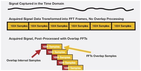
Figure 17. Illustration of overlap processing.
As shown in this picture, when a frame of new data is acquired after passing the Acquisition Mode control, only a portion of the new data will be used. Overlap calculation will speed up the calculation with the same target average number. The percentage of overlap is called overlap ratio. 25% overlap means 25% of the old data will be used for each spectral processing. 0% overlap means no old data will be reused.
When two signals are from different units—and because the sampling rate of two systems is slightly different--there will be a different number of sample points for the same duration of acquisition. Therefore, we cannot simply use the overlapping ratio to calculate the starting point of the block for each channel. Instead, we will calculate the starting points of two channels with the following algorithm:
Use the same algorithm based on block size and the overlapping ratio to calculate the starting point of the first channel (X channel).
To calculate the starting point of the block of the second channel (Y channel), using time stamps, we look for the point that is nearest to the starting point of the first input channel in absolute time. Assume the time difference between these two points is dt:
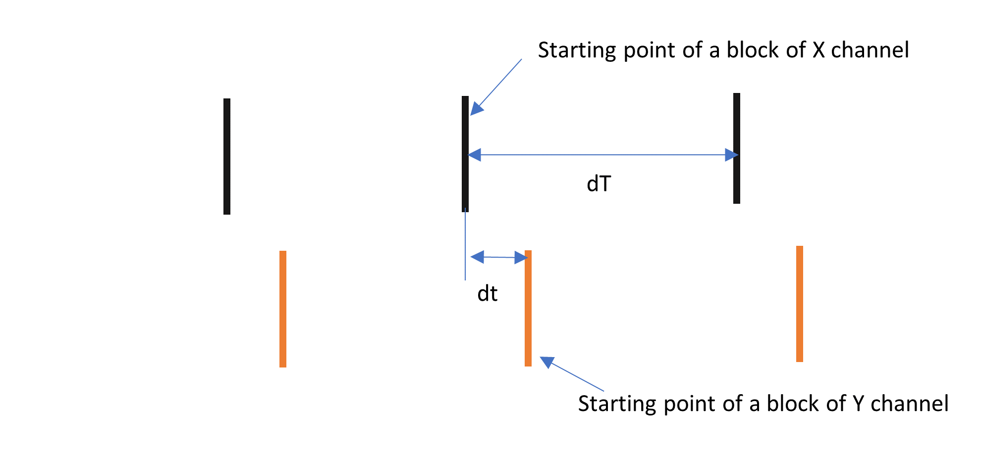
Figure 18.
With the starting points of both channels known, calculate the instantaneous cross spectrum between two channels, Syx = Sx* Sy * T, using the same formula:
https://www.crystalinstruments.com/dynamic-signal-analysis-basics
Cross Spectrum Computation
Figure 19.
Cross spectrum or cross power spectrum density is a frequency spectrum quantity computed using two signals, usually the excitation and response of a dynamic system. Cross spectrum is not commonly used on its own. Most often it is used to compute the frequency response function (FRF), transmissibility, or cross correlation function.
Follow the steps below to compute the cross-power spectral density Gyx between channel x and channel y:
Step 1 - compute the Discrete Fourier Transform of input signal x(k) and response signal y(k):

Step 2 - compute the instantaneous cross power spectral density:
Syx = Sx * Sy * T
Step 3 - average the M frames of Syx to obtain the averaged cross power spectrum: Gyx
Gyx = average (Syx)
Note: there are many ways to average the spectrum, including linear average, moving linear average, exponential average etc. Regardless of the method used, the same method should be applied to both auto and cross spectra in order to compute the transfer and coherence functions.
Step 4 - Compute the energy correction and double the value for the single-sided spectra.
Gyx = 2 Gyx/EnergyCorrection
After the cross spectrum is calculated, the system transfer function (H1 type is shown here) can be derived by:
Hyx = Gyx / Gxx
Where Gxx is the averaged auto-power spectrum.
Apply the phase correction to cross spectrum Syx[n]
With time stamped signals, the cross spectrum and transfer function calculation process will remain the same except that we will add a phase correction process after the instantaneous cross spectrum is calculated.
Syx is called instantaneous cross spectrum because it has no average effect in it. It is an array with N pairs of complex numbers and its nth element is Syx[n]. After Syx is calculated, we will conduct a phase correction to each point of the signal Syx[n].
We know the data from two input channels has a known time delay of dt. The phase correction formula will apply the following phase change to each element:
Phase change[n] = 2π * (dt/dT) * n/N
Where:
- dt is the time delay between the starting point of the block of Y channel vs. X channel
- dT is the nominal sampling interval. For example, for a sampling frequency of 102.4 kHz the dT is 9.765625 µs.
- n is the index number of the element in the array
- N is the total size of the array
The formula above simply indicates that if the time delay is 1 sample point long, the phase shift between two channels will be 2π, or 360 degrees, when the frequency index is equal to the sampling frequency. The following figure shows how it can be described in the frequency domain:
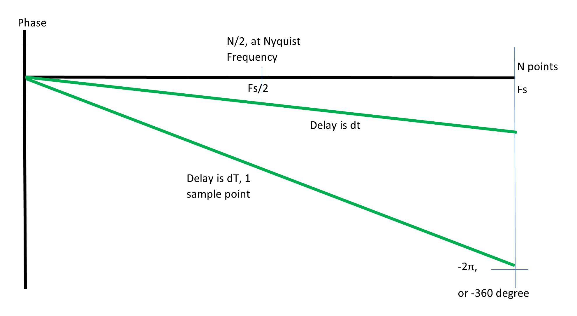
Figure 20.
Now, the question is how to make a phase correction to a complex number.
If a complex number is expressed in an amplitude and its phase, we can simply add the Phase change[n] value to the phase portion θ.
![Phase change[n] value](https://images.squarespace-cdn.com/content/v1/5230e9f8e4b06ab69d1d8068/a0a2128a-e1c1-4f91-9f89-57cc7417baa5/complex+number)
Figure 21.
But if the complex number is expressed in real and imaginary parts, you will have to transform them into amplitude/phase, add phase, then transform it back to real/imaginary parts.
Conduct the average and remaining spectral calculations
After the phase correction is made to the instantaneous spectrum Syx, it will be averaged into Gyx, the averaged cross spectrum, using either a linear or exponential averaging algorithm. Then all other spectra, FRF, Coherence etc., can be calculated as usual.
Data processing diagrams
The GRS data acquisition systems can be physically separated by hundreds of feet or miles without electrical hardware connections. The systems will instead receive GPS signals from the satellites and certain commands from a remote computer through wireless communication methods.
The general data flow using time stamped signals is described in the following figure.

Figure 22.
The processing block at the bottom, Spectral Analysis for time stamped signals, can be expanded to following diagram:
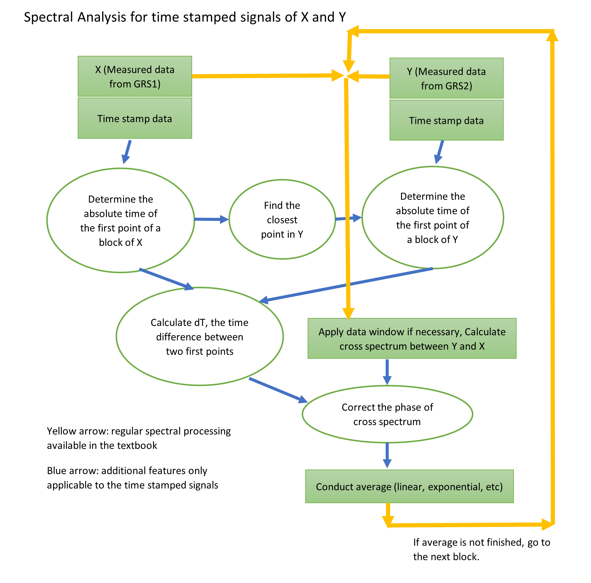
Figure 23.
The interesting part of this technique is that while the misalignment of sampling clocks in the time domain is obviously caused by deviations of the ADC sampling clocks from two data acquisition units, the correction is not performed in the time domain. Instead, it is performed in the frequency domain of cross spectrum. In fact, we believe that there is no good algorithm to correct the arbitrary time delay between X and Y channels with two separate ADC clocks.
Longest useable GPS antenna cable length for GRS and CoCo-80X
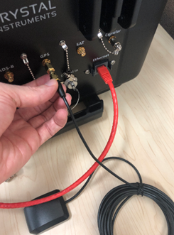
Figure 24.
Certain applications prohibit the hardware from accessing signals sent from the GPS satellites. A longer antenna cable is required.
CI has tried several antenna models with different lengths. The longest tested antenna meeting the requirement was 150 feet long. This test indicated that the data acquisition units can be positioned in a location that has no direct exposure to the GPS signals as long as the terminal of its GPS antenna was accessible to the GPS signals.
GPS Repeater used for Indoor Test
The GPS signal is not always directly accessible when conducting tasks inside a building. Instances arise where a device might be situated in an area with inadequate GPS signal strength, preventing proper timestamping of measured signals. To address this challenge, a potential solution involves strategically placing an antenna in a location with strong GPS signal reception. The received signal can then be routed through a cable to a GPS repeater, which not only amplifies but also transmits the signal across its vicinity, effectively mitigating the signal quality issue.
CI has tested several brands of GPS repeaters and they all work as published. One tested model was the ROGER™ GNSS from Roger -GPS Ltd, Finland. (https://www.gps-repeating.com/frontpage.html )
A single ROGER™ GNSS Repeater is enough to provide a GNSS indoor coverage area about 1 to 1600 square meters. The modern receivers can detect the signal at a level less than -160 dBm, such like TETRA radios and smart phones using A-GPS (Assisted GPS), so the distance can reach up to 50 meters from the repeater’s center. Several ROGER™ GNSS Repeaters can be installed in the same building. Alternatively, the signal coverage provided by a single package can be extended with ROGER™ GNSS additional products such as line amplifiers and signal splitters.
Examples of Applications
Bare-wire testing
To validate the effectiveness of the algorithm above, we established the following test. We took two GRS units, each with the GPS time stamping function installed. We fed white noise into one channel of GRS unit 1 and one channel of GRS unit 2. The same white noise source can be split into two using a simple BNC splitter.

Figure 25.
We set both GRS units with a nominal sampling rate of 102.4 kHz and started to acquire the data. All measurement data can be recorded into the SD card. By design the total recording duration can be hundreds of hours, but we only recorded a few minutes for this particular test.
After the recording, we transmitted the measured data files together with their time stamp files to a PC using GRS-Host software. The GRS-Host software can directly read the data files on the SD card or read the data files from each GRS when Ethernet is connected.
After the data files are located on the PC, we opened the Post Analyzer software (PA). PA can merge multiple data files into one and then analyze it.
After the measured data files are merged based on time stamping information, they can be analyzed using the technique mentioned above. In order to demonstrate the effectiveness of this method, we set the average number to 1, which means no averaging over multiple blocks of data. If we apply averaging, then the phase measurement will not be valid.
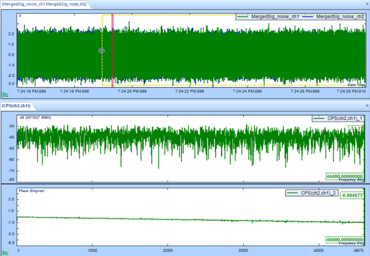
Figure 26.
The screenshot above shows a typical test result. The top trace shows the original time data from both GRS and CoCo units. The middle trace shows the amplitude of the cross-spectrum of this particular block. The bottom one, which is what we really care about, shows the phase spectrum of this block from 0 Hz to 46 kHz. A cursor located at 46 kHz has a value at -0.984675 degree. This is the phase measurement at this frequency.
In order to establish a statistical confidence of the phase deviation, we calculated thousands of blocks cross-spectra and stored all of their phase values at 46 kHz. After these values are stored, a histogram like the following can be drawn:
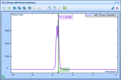
Figure 27.
In this histogram plot, the vertical axis indicates the block counts, i.e., the number of phase measurements at 46 kHz. The horizontal axis is the phase in degrees. By measuring thousands of frames of cross-spectra, we are able to determine the statistical distribution of the phase error. This is how we can claim the phase measurement accuracy as below:
| Phase match between two independent units: |
±5°(degree) at 40 kHz ±2.5°(degree) at 20 kHz ±0.5°(degree) at 2 kHz |
We used multiple GRS and CoCo units for testing, and they all demonstrated similar characteristics.
The phase value can be converted directly to the time delay of that frame between two channels. The formula is:
dT = 1/46 kHz * phase/360
For example, if the phase is 5 degrees, then the time delay between two channels of that frame is:
dT = 1/46 kHz * 5.0/360 = 3e-7 (second) = 300 ns
Calculating the auto-spectrum is relatively easy because it only needs to deal with the data from a single channel. Once auto-spectra and cross-spectrum are calculated, we can compute the Frequency Response Function and the coherence function as shown above.
Testing results using an electrical simulation box
Crystal Instruments developed an electrical simulation box to simulate the resonance of a structure. It is a perfect tool to validate the effectiveness of the time stamped signal processing algorithm.
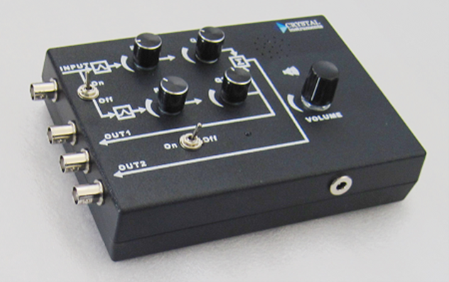
Figure 28.
By connecting the simulation box to a signal analyzer with random excitation, we are able to measure the transfer function (FRF).

Figure 29.
In order to validate the effectiveness of Time Stamped Signal Process described in this document, we can connect two GRS units to acquire the data:
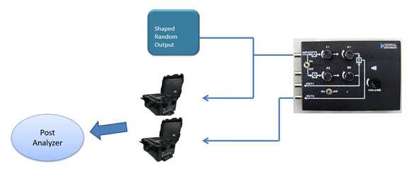
Figure 30.
With two different methods of measurement, we can calculate the FRF and make the comparison:
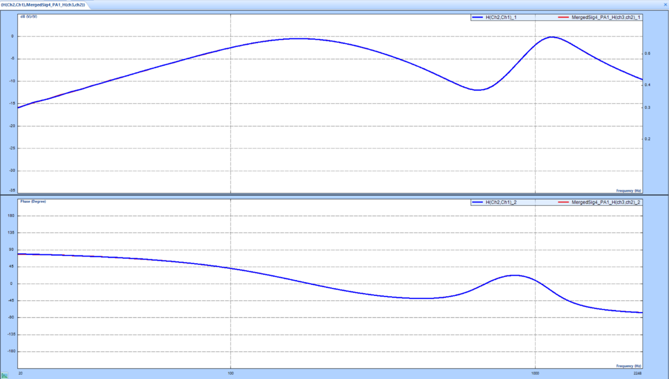
Figure 31.
Blue: FRF measured using single Spider instrument
Red: FRF measured with two GRS units, using Time Stamped Signal Processing (the red signals in the plot above are nearly invisible because they are covered by the blue ones).
The two measurement signals are nearly identical. This comparison further proves that the Time Stamped Signal Processing can generate the same results as using one single instrument.
Modal Testing
Objective
A Frequency Response Function (FRF) is first calculated using a conventional instrument, the Spider system. Its testing results are compared to those obtained using two separate systems, one system measures excitation and one system measures response. While the test is conducted on a small structure, the method is applicable to any large mechanical structures such as vessel ships, bridges, or buildings.
Test Results
FRF Measurement using Hammer Impact Modal Test on a Plexiglass Plate
1. A hammer impact modal test is carried out on a plexiglass plate for one measurement point.
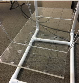
Figure 32.
2. The raw time stream data for the excitation is recorded on one GRS system. The raw time stream data for the response is recorded on the second GRS system. This data is later transferred to PA software for post-processing and calculating the FRF.
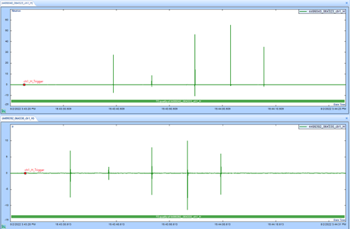
Figure 33.
3. The Spider system also measures the excitation from the hammer impulse and the response from the accelerometer response. The FRF is calculated using EDM Modal software.

Figure 34.
4. The configuration settings are appropriately set and are kept consistent across the different hardware systems and EDM software.
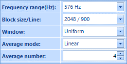
Figure 35.
5. The FRF plots are overlaid to compare the data from the GRS and Spider system. The green curve is generated using the Spider-80X’s acquired data and the blue curve is generated using the data acquired from the two GRS systems.
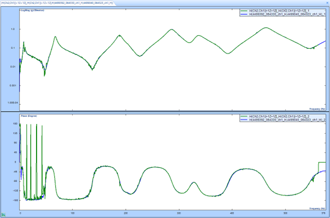
Figure 36.
This test indicates that with two separate acquisition units, we can measure the FRF and other modal parameters and obtain results identical to using conventional instruments while the latter has to be wired and has the limitation of distance between their measurement points.
Sound source identification (locating the coordinates of a gunshot)
If the earth is flat, we would only require three data acquisition units to measure the sound of a gunshot and thereby determine the location of its shot. If the assumption is that the earth is not flat, four acquisition units will be required to determine the location of the sound source.
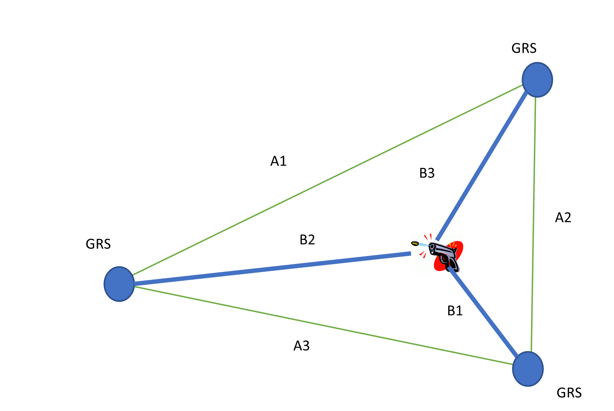
Figure 37.
Known: locations of A1, A2, A3 (GPS on GRS can provide very accurate location information)
Known: distance of B2-B1, B3-B2, B3-B1 (the difference between any pair). These can be measured using correlation functions of any pair of sound pulses. These distances can be estimated by following method:
Use any pair of time domain signals, with time stamps, calculate the cross-correlation.
Using cross-correlation, detect the peak location.
Based on peak location, determine the time delay between two signals.
Based on time delay and the speed of sound, determine the distance.
Then the position of origin of the sound can be calculated.
If the three acquisition units and the sound source are not in the same plane, we will need the fourth acquisition unit to determine its location. A simple software was developed based on the cross-correlation method to calculate the delay between each pair of acquisition units. The sound source location can be calculated with these three time-delays and the assumed speed of sound.

Figure 38.
In the summer of 2022, CI conducted a successful test at the Los Altos Rod and Gun Range in Los Gatos, California. The results were excellent. Below is a screen shot of three signals overplotted on the same window.

Figure 39.
Using the recorded signals, we used cross-correlation methods to calculate the location of the gunshot source. It can be accurately displayed on the map as shown below:

Figure 40.
For details regarding this test, please contact Crystal Instruments to request more information.