
Understanding Random Vibration Signals
Download PDF | © Copyright Crystal Instruments 2016, All Rights Reserved.Verifying the robustness of products (or their packaging) by subjecting them to shaker-induced vibration is an accepted method of “improving the breed”. While shock bumps and sine sweeps are intuitively obvious, random shakes with their jumps and hissing are anything but. Even the language of a random test is confusing at first meeting. Let’s try to improve upon that first introduction to random signals!
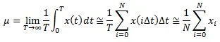
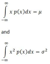
To start with, a random time-history is simply a signal that cannot be precisely described by a simple equation in time; it can only be described in terms of probability statistics. Two of the most important of these statistics are the mean and the variance. The mean, μ, is the central or average value of a time history, x(t). It is the DC component of the signal and is defined by the equation:

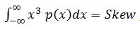
The variance, σ2, is the averaged (unsigned) indication of the signal's AC content, its instantaneous departure from the mean value. It is defined by:
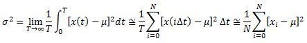
The square root of the variance, σ, is termed the standard deviation.
These functions are closely related to a third time-domain statistic, the mean-square, defined as:
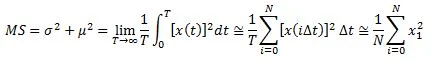
The square root of the mean-square is the familiar root mean-square (RMS) value, commonly used to characterize AC voltage and current, as well as the acceleration intensity of a random shake test. Because these statistics are so frequently measured from signals with a zero-valued mean (no DC), the differentiation between standard deviation and RMS and between variance and mean-square has become unfortunately blurred in modern discussions.
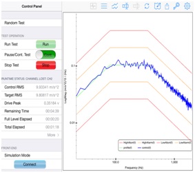
The Control spectrum you measure during a random shake test is also a statistical description. The measured variable is (normally) the output of an accelerometer mounted to the shaker table. The sensor's voltage output is scaled to engineering units of acceleration, typically gravitational units (g's) and sampled at a fixed interval, Δt. This time-sampled history is transformed to the frequency domain using the Fast Fourier Transform (FFT). In this process, a series of "snapshots" from the continuous time waveform are taken and dealt with sequentially.
Each snapshot is multiplied by another sampled time history of the same length, called a window function. The multiplied window function serves to smoothly taper the beginning and end of each time record to zero, so that the product appears to be a snapshot from a signal that is exactly periodic in the N Δt samples observed. This is necessary to preclude a spectrum-distorting convolution error that the FFT would otherwise make. The resulting discrete complex spectrum has nominal resolution of Δf = 1/NΔt and g amplitude units. However, every spectral amplitude computed is actually greater than what would result from detecting the amplitudes of a bank of perfect "brickwall" analog filters of resolution Δf.
Each complex spectrum is prepared for averaging by multiplying each complex amplitude it by its own conjugate. This results in a real-valued "power" spectrum with g2 amplitude units. To correct the over-estimated amplitude, each squared magnitude is divided by the equivalent noise bandwidth, kΔf (Hz) of the filters synthesized by the FFT. The value of the constant, k, is determined by the shape of the window function. The most common of these is called a Hann window (sometimes Von Hann or Hanning) for which k equals 1.5. The resulting amplitude units are now g2/Hz and the spectrum is said to have Power Spectral Density scaling.
The final step in the process is to ensemble average the current spectrum with all of those that have preceded it. The resulting average is called a Power Spectral Density (PSD) and it has the (acceleration) units of g2/Hz. The averaging is done using a moving or exponential averaging process that allows the averaged spectrum to reflect any changes that occur as the test precedes, but always involves the most recent DNΔt/2 seconds of the signal. D is the specified number of degrees-of-freedom (DOF) in the average, numerically equal to twice the number of (non-overlapping) snapshots processed.
If the snapshots are taken frequently enough not to miss any time data, the process is said to be operating in real time (as it must to control the signal's content). If the process runs faster, the snapshots can actually partially overlap one-another in content. When the successive windows overlap, the resulting complex spectra contain redundant information. The degrees-of-freedom setting is intended to specify the amount of unique (statistically independent) information contained in the averaged Control spectrum. When overlap processing is allowed, the number of spectra averaged must be increased by a factor of [100/(100-% overlap)] to compensate for this redundancy.
The resulting PSD describes the frequency content of the signal. It also echoes the mean and the variance. The (rarely displayed) DC value of the PSD is the square of the mean. For a controlled acceleration (or velocity) shake, this must always be zero - the device under test cannot depart from the shaker during a successful test! Since the mean is zero, the RMS value is exactly equal to the standard deviation, σ. The area under the PSD curve is the signal's variance (its "power"), σ2. The term power became attached to such "squared spectra" when the calculation was first applied to electrical voltages or currents. (Recall that the power dissipated by a resistor can be evaluated as i2R or E2/R.)
It bears mentioning that long before real-time control of a random vibration signal was possible, random vibration test were conducted using a "white- noise" generator and a manually adjusted equalizer to shape the spectrum. Filter-based signal analysis was employed with a human "in the loop" to achieve some semblance of spectral control. In that same era, the PSD was formally defined by the classic Wiener-Khintchine relationship as the (not very fast!) Fourier transform of an Autocorrelation function. An autocorrelation is defined by the equation:
In essence, the autocorrelation averages the time history multiplied by a time-delayed image of itself. The symmetric function of time that results was often used to detect periodic components buried in a noisy background. The "squaring" of an autocorrelation would reproduce the periodic signal with greater amplitude, rising above the random noise background. In the process, it echoed the signal's mean and variance. When you autocorrelate x(t), the Rxx(τ) amplitude at lag time τ= 0 is equal to σ2 + μ2. As the lag time approaches either plus or minus infinity, the correlation amplitude collapses to μ2. Thus if the signal is purely random, the autocorrelation amplitude varies smoothly between the mean-square and the square of the mean.
Clearly, the mean and variance dominate statistical measurements in both the time and frequency domains. They are also reflected by so-called amplitude domain measurements. The most basic of these is called a histogram. To measure a histogram, break a signal's potential amplitude range into a contiguous series of N amplitude categories (i.e. x is between a and b) and associate a counter with each category. Initialize the measurement process by zeroing all of the counters. Take a sample from the time-series in question, find the category its amplitude fits within and, increment the associated counter by one. Repeat this action thousands of time. Plot the counts retained (vertically) against their category amplitude (horizontally). You have just measured a histogram.
A histogram may also be used to graphically present tabular measurements from an experiment or even gaming odds. For example, consider tossing dice. If you toss a single (honestly constructed) die, any one of its six numbered faces may face up and the odds are 1 in 6 that any specific number will be rolled. As a histogram, this amounts to 1 count for each of the possible tossed numbers, 1 through 6, a rectangular distribution. Now consider rolling two dice (or one die twice) and recording their sum. There are now 36 possible combinations that might be rolled with sums spanning 2 to 12. However, the 11 different possible sums are not equally probable. There are six combinations totaling 7, five totaling either 6 or 8, four totaling 5 or 9, three totaling 4 or 10, two totaling 3 or 11 and only one way to roll either a 2 or a 12. The histogram now takes on a triangular shape. Finally, consider what happens when you roll three dice. The number of combinations increases to 216 with 16 different possible sums. The likelihood of a 10 or 11 is 27 times as probable as rolling a 3 or an 18. With three dice in the game, the histogram takes on a bell-shaped curve. These three histograms are plotted below for comparison.
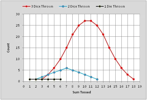
The three histograms have different independent-variable spans. If we choose to plot the averaged (mean) number tossed instead of the sums, we can align the three histograms horizontally, making comparisons between the three plots simpler. If we now change the vertical scale of each trace so that each curve bounds a (dimensionless) unit area, we have converted the three histograms to Probability Density Functions (PDF). Note that if the independent variable (horizontal axis) carries an engineering unit, the vertical (probability density) axis must bear the reciprocal of that unit to render the bounded area dimensionless.
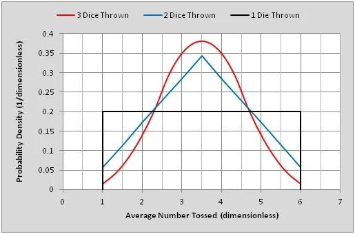
Several important things happen when a histogram is scaled as a probability density function. Since the area under this p(x) curve is 1.0, and the curve spans all known possibilities of the independent variable, x, it may be used to evaluate the probability of x falling between two known bounds, say Xa and Xb.
That is, since
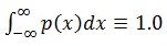
the probability that -∞ ≤ x ≤ ∞,
The definite integral
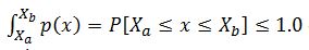
defines the probability that x is between Xa and Xb in value.
Of equal importance, the first two integral moments of the PDF return the mean and variance of the signal p(x) characterizes. Specifically:
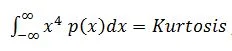
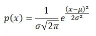
Two higher moments are pertinent to controlled random vibration tests. These are:
a measure of the signal’s amplitude symmetry (about the mean) and
which describes the spread of the extreme-amplitude “tails” of the PDF.
Before we continue, reflect for a moment on the three PDFs plotted from our dice-throwing model. Note the rapid convergence from a rectangular PDF towards a bell-shaped one as independent variables are added or averaged together. This clear progression is observed in all manner of natural phenomena. Since most occurrences involve the summation or integration of many independent component happenings, many things in nature tend to have bell-shaped PDFs. Pass a signal of almost any PDF shape through a filter or averaging process (be it electrical or mechanical) and the output will tend strongly to the naturally occurring mean-centered symmetric bell curve.

Johann Carl Friedrich Gauss (1777-1855) had a strong and intuitive understanding of this natural tendency. He proposed a mathematical model for the bell-shaped p(x) that has stood the test of centuries and is at the center of our understanding of random signals and variables. His classic definition for p(x) is:
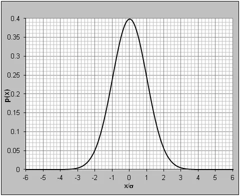
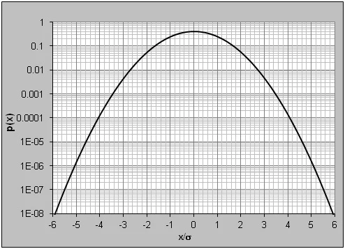
The classic Gaussian PDF is plotted above. Note that the "tails" actually extend to ±∞. To appreciate this point, we repeat the Gaussian PDF plot using a logarithmic vertical axis. This scaling is frequently done in vibration work, but rarely shown in statistic texts.
If an experimental measurement matches the Gaussian PDF model, the Gaussian model can then be used to draw many important inferences about the measurement. Many statistical curve-matching tests are available to establish if a measurement is Gaussian. These include the Kolmogorov-Smirnov (KS), Shapiro-Wilk and Anderson-Darling tests. For practical purposes, most well-fixtured and well-conducted random shake tests will produce data that pass any of these model-matching statistical tests for Gaussian behavior.
Important conclusions that result from deeming a measured Control acceleration Gaussian include:
- The random Control acceleration signal spends 68.3% of its time within ± 1σ, 95.5% within ± 2σ, and 99.7% within ± 3σ. For practical purposes, the signal has a crest factor (peak to RMS ratio) of 3.
- The Skew is μ(3σ2 + μ2)=0 (as μ is 0)
- The Kurtosis is 3σ4 + 6σ2μ2 + μ4 = 3σ4 for the same reason)
Further, we find that if a time-history is Gaussian, the real and imaginary components of its Fourier Transform are also (independently) Gaussian distributed variables. Further, the vector resultant magnitude of those Gaussian components exhibits a different PDF; the spectral magnitude is Rayleigh distributed. Of far greater interest is that the sum of the squares of the real and imaginary components (the power spectrum magnitude) is a Chi-square (χ2) distributed variable, as is the variance
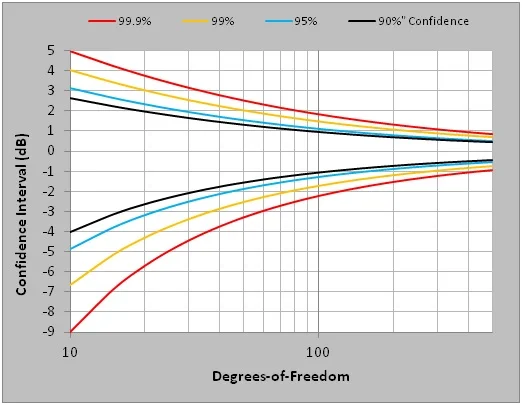
Knowing that the Control PSD has χ2 distributed spectral magnitude allows construction of a confidence interval about any g2/Hz value. The curves above illustrate statistically reasonable bands of variation (±dB) for a g2/Hz spectral value with regard to two variables: Confidence and Degrees-of-Freedom. Statistical Confidence is usually expressed as a percentage. For example, 99.9% Confidence is shorthand for saying 99.9% of the spectral Lines in a PSD will be within the curve-specified upper and lower bounds. So if you average using 200 DOF, you are 90% certain that all of your PSD measured magnitudes are correct within ± 1 dB.
We have just begun to scratch the surface of the things that can be learned and ascertained about random signals with Gaussian mean and Chi-square variance. But, that is the stuff of future postings!