
Basic Theory of Frequency Response Function (FRF)
Download PDF | Sandeep Mallela - Senior Product Manager | © Copyright Crystal Instruments 2020, All Rights Reserved.
A common application of dynamic signal analyzers is the measurement of the Frequency Response Function (FRF) of mechanical systems. This is also known as Network Analysis, where both system inputs and outputs are measured simultaneously. With these multi-channel measurements, the analyzer can measure how the system “changes” the inputs. If the system is linear, which is a common assumption, then this “change” is fully described by the Frequency Response Function (FRF). In fact, for a linear and stable system, the response of the system to any input can be predicted just by knowing the Frequency Response Function.
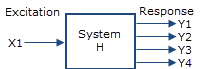
Broadband random, sine, step or transient signals are widely used as excitation signals in test and measurement applications. Figure 1 illustrates that an excitation signal x, can be applied to a UUT (Unit Under Test) and generate one or multiple responses denoted by y. The relationship between the input and output is known as the transfer function or frequency response function and represented by H(y,x). In general a transfer function is a complex function that describes how the system modifies the input signal magnitude and phase as a function of the excitation frequency.
With various excitations, the characteristics of the UUT system are measured experimentally. These characteristics include:
Frequency Response Function (FRF), which is described by:
Gain as a function of frequency
Phase as a function of frequency
Resonant Frequencies
Damping factors
Total Harmonic Distortion
Non-linearity


Figure 1: Left - a UUT with one response; Right - a UUT with two responses
Frequency response is measured using the FFT, cross power spectral method with broadband random excitation. Broadband excitation can be a true random noise signal with Gaussian distribution, or a pseudo-random signal of which the amplitude distribution can be defined by the user. The term broadband may be misleading, as a well implemented random excitation signal should be frequency band-limited and controlled by the upper limit of the analysis frequency range. That is, the excitation should not excite frequencies above that which can be measured by the instrument. The random generator will only generate random signals up to the analysis frequency range. This will also concentrate the excitation energy on the useful frequency range.
The advantage of using broadband random excitation is that it can excite the whole frequency range in a short period of time so the total testing time is less. The drawback of broadband excitation is that its frequency content is spread over a wide range within a short duration. The energy contribution of the excitation at each frequency point will be much less than the total signal energy (roughly, it is -30 to -50dB less than the total). Even with a large average number for the Frequency Response Function (FRF) estimation, the broadband signal will not effectively measure the extreme dynamic characteristics of the UUT.
Swept sine measurements, on the other hand, optimizes the measurement at each frequency point. Since the excitation is a sine wave, all of its energy is concentrated at a single frequency, eliminating the dynamic range penalty in a broadband excitation. In addition, if the frequency response magnitude drops, the tracking filter of the response can help to pick up extremely small sine signals. Simply optimizing the input range at each frequency can extend the dynamic range of the measurement to beyond 150 dB.
Measure the Frequency Response Function Using Swept Sine
A sine signal with a fixed frequency is expressed in the following Frequency Response Function formula as:
x(t) = sin(2πf0 t)
where t represents time. A sweeping sine signal has a changing frequency that is usually bound by two limits. The frequency change can be either in the linear scale or logarithmic scale based on different user requirements. The swept sine signal can be defined by the following parameters:
- The low frequency boundary, which is simply called Low Frequency or fLow
- The high frequency boundary, which is simply called High Frequency or fHigh
- The sweeping mode, either logarithmic or linear
- The sweeping speed, in either octave/min if the sweep mode is logarithmic, or in Hz/Sec if the sweeping mode is linear
- The amplitude of the sine signal, A(f, t), which can be a constant or a variable of time and frequency.
x(t) = A(f,t) * sin (2π ∙ f (fLow,fHigh,Speed) ∙ t )
The instantaneous frequency f(fLow,fHigh,Speed) represents the current frequency of the sweeping sine. It is a changing variable and usually displayed on the screen as Sweeping Frequency.
The Sweeping frequency can also be manually controlled during the test with the Hold, Resume, Jump or Pause controls.
Unlike some Digital Signal Analysis (DSA) products which use swept sine test with multiple discrete stepped sine tones in a sequence, the CI swept sine test uses a true digital synthesizing technique to generate sine sweeps with extreme analog-like smooth transition from one frequency to another. This ensures that there are no sharp transitions during the test that might shock the UUT. Figure 2 shows a typical swept sine signal with 1.0 Vpk.
A swept sine can sweep in either linear or logarithmic mode. Linear sweep means the frequency will change at a constant speed, with units of Hz/sec. In this case the sweep rate is constant and the same at all frequencies. Alternatively, the sweeping mode can be set as logarithmic or Log. In Log mode, the sweeping speed is slower at low frequencies and faster at higher frequencies. In Log mode, the sweeping speed units are in Octave/Min.

Figure 2. Typical digitally synthesized swept sine signal.
Capability of Measuring and Displaying Hundreds of FRF Signals
In the PC FRF, FRF signals are calculated by the PC instead of the Spider. Since the PC FRF relies on the PC's resource which is much more powerful than the Spider's processor, hundreds of FRF signals can be computed simultaneously without consuming the Spider's resource. Multiple channels can be specified as reference channels.
The relationship between input (force excitation) and output (vibration response) of a linear system is given by:
{Y} = [H]{X}
where {Y} and {X} are the vectors containing the response spectra and the excitation spectra, respectively, at the different DOFs in the model, and [H] is the matrix containing the FRFs between these DOFs.
The equation above can also be written as: 
where Yi is the output spectrum at DOF i, Xj is the input spectrum at DOF j, and Hij is the FRF between DOF j and DOF i. The output is the sum of the individual outputs caused by each of the inputs.
The FRFs are estimated from the measured auto- and cross-spectra of and between inputs and outputs. Different calculation schemes (estimators) are available in order to optimize the estimate in the given measurement situation (presence of noise, frequency resolution, etc...).
For the classical case of a single input, the equation above gives the output at any DOF i, with the input at DOF j, as:
Yi = HijXj or Hij = Yi/Xj
since the input is zero at all the DOFs other than j.
The FRF Hij can be estimated using the various classical estimators such as:
H1 = Gxy/Gxx
or
H2 = Gyy/Gyx
where Gxx and Gyy are the auto spectra of input and output respectively, Gxy is the cross-spectrum between input and output, and Gyx is the cross-spectrum between output and input (i.e., the complex conjugate of Gxy). H1 has the ability, by averaging, to eliminate the influence of uncorrelated noise at the output, whereas H2 has the ability, by averaging, to eliminate the influence of uncorrelated noise at the input. Compared to H1, H2 is less vulnerable to bias errors at the resonance peaks caused by insufficient frequency resolution (called resolution-bias errors).
The Spider is capable of measuring and displaying hundreds of FRF signals simultaneously. Users can manually create a list of FRFs by constantly changing the excitation and response channels to generate all possible combinations of FRF signals.
Recommended for FRF Measurement
The CoCo-80X (and CoCo-90X) handheld dynamic signal analyzers are recommended by Crystal Instruments for frequency response function (FRF) measurement.
PC-based real time solutions include Crystal Instruments Spider-80X, Spider-80Xi, and Spider-20 systems.