
Multi-Resolution Spectrum Analysis
Download PDF | By James Zhuge, Ph.D. - Chief Executive Officer | © Copyright Crystal Instruments 2019, All Rights Reserved.
Introduction
Many problems in mechanical structure and acoustic applications ask for a spectrum analysis method generating the frequency values with non-uniform frequency resolution. In these applications, it is preferable to use a logarithmic distribution in the frequency axis, i.e., the lower frequency band should have a finer frequency resolution than the higher frequency band. We will show a few examples after the introduction.
In the CI Product Note 001, Dynamic Signal Analysis Basics (Reference 2), we discussed how various spectra are calculated. These include the Linear Spectrum, Auto Spectrum, Cross Spectrum, Phase Spectrum, Coherence Function and Frequency Response Function. In modern day products, all of these spectra are calculated based on the Cooley–Tukey FFT (Fast Fourier Transform) algorithm (Reference 1). The basic formula of discrete Fourier transform is:
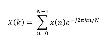
where
x(n) samples of time waveform
n running sample index
N total number of samples or “frame size”
k finite analysis frequency, corresponding to “FFT bin centers”
X(k) discrete Fourier transform of x(k)
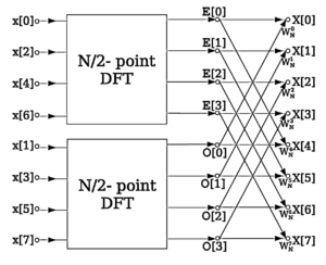
In most cases, a Radix-2 DIF FFT algorithm is used, which requires that the total number of samples be a power of 2 (total number of samples in FFT = 2m, where m is an integer.)
A distinct feature of FFT is that it will create a uniform resolution across the whole range in the frequency domain by transforming the time domain signal, which is sampled uniformly. The frequency resolution, dF, is the inverse of T, the total duration of the time block signal being transformed.
For example, if the FFT is applied to a block of time signal with duration of T = 0.5 seconds, the frequency resolution between each adjacent bins will be 1/(0.5 sec) = 2Hz across the whole range.
The frequency resolution of all the spectra calculated based on FFT shall be uniformly distributed across the range of analysis. The resolution at 10Hz is the same to that at 1000Hz. This creates a problem when the analysis objects require a non-uniformed frequency resolution, as the FFT-based spectrum analysis does not fit well.
The computational cost of DFT is on the order of N*N where N is the block size of the time signal while that of FFT is on the order of O(N log N).
One might ask: what if the FFT was not invented by Cooley and Tukey in 1965? Then people would be using the much lower efficiency algorithm, the Discrete Fourier Transform (DFT), to compute the spectrum. The advantage of DFT is that the resolution of the frequency spectrum does not need to be uniformly distributed. In fact, the frequency resolution can be arbitrarily distributed when DFT is calculated. It appears that DFT is a better approach than FFT because it can provide the bins (frequency lines) at any frequency point in the spectrum. However, the tradeoff for using DFT is that the cost of computation is too high.
It would be revolutionary if we could identify a method that both maintains the computational efficiency of FFT efficiency, and creates a frequency spectrum compatible with non-linear distribution of the resolution (particularly with logarithmic distributions).
After over twenty years of research and development, Crystal Instruments successfully introduced and implemented the so-called multi-resolution spectrum analysis in many lines of its products, including CI Random vibration controller, dynamic signal analyzer and modal data acquisition. The multi-resolution spectrum analysis solves the problem mentioned above with enormous benefits. This paper shows how it was realized and example results.
Uses Cases for Non-Uniform Frequency Resolution
In this section, we present a few examples when non-uniform frequency resolution is required.
Music Frequencies
The frequencies of different pitch tunings on a typical keyboard of the piano is evenly distributed on the logarithmic scale instead of the linear scale:

The characteristics of music tones of any other instruments has the similar frequency distribution. Human hear the tones of sound and differentiate them according to their frequency ratio, which is easily described in the log scale.
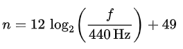
The following equation gives the frequency f of the nth key, as shown in the table:
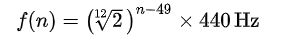
(a' = A4 = A440 is the 49th key on the idealized standard piano)
Alternatively, this can be written as:
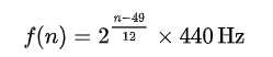
Conversely, starting from a frequency on an ideal standard piano tuned to A440, one obtains the key number by:
If a user wants to use a dynamic signal analyzer to measure the time domain signal of the piano sound and provide an accurate estimation of the frequency when a tone sounds, it would require much finer resolution at 27.5Hz than that at 1760Hz because human ear compares two tones by multiplicative ratio instead of additive difference.
If the frequency resolution of the spectrum analyzer is the same, say 1.0Hz, it will result in less than 0.1% of error of a frequency reading of 1760Hz while the error at 27.5Hz can be as large as 3%. This example shows that it is better to design a signal analyzer that can provide a frequency resolution that is uniformly distributed in logarithmic scale rather than linear scale, which the FFT provides.
Damping Estimation for Resonance Frequencies
The structure vibration can be decomposed into multiple simple models, where the system's equation of motion is
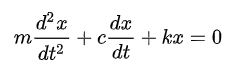
and the corresponding critical damping coefficient is
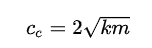
or

where

is the natural frequency of the system.
Using the natural frequency of
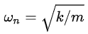
and the definition of the damping ratio above, we can rewrite this as:
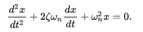
The damping ratio ζ is dimensionless, being the ratio of two coefficients of identical units.
Damping is often a dominant factor for its dynamic behavior. The damping ratio ζ determines the intensity of the resonant oscillation, which can be measured by the amplitude of the frequency response function. While the damping ratios of all resonances vary, they are mainly determined by the material of the objects. For example, plastic will have a much higher damping ratio than steel. In other words, the damping ratio of a given material will always fall into a certain range.
The table below shows the range of viscous damping ratio ζ for certain materials, taken from V. Adams and A. Askenazi (Reference 3):
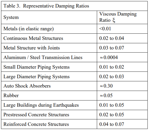
This table documents the damping ratio ranges for certain specified materials.
Now let’s look at how the damping ratio is estimated with an FFT dynamic signal analyzer. With FFT signal analyzer, the Frequency Response Function (FRF) between response and excitation can be estimated. Usually the response is an acceleration signal measured by a transducer mounted on the structure. The excitation signal is the force applied to the structure by either an impact hammer or a shaker.
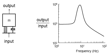
The FRF can be estimated by the method described in Reference 2. A typical FRF plot including both amplitude and phase will look like this:
A classic method for determining the damping ratio ζ at a resonance in a Frequency Response Function (FRF) is to use the “3 dB method” (also called “half power method”).
In a FRF, the damping is proportional to the width of the resonant peak about the peak’s center frequency. By looking at the three dB down from the peak level, one can determine the associated damping.

The “quality factor” (also known as “damping factor”) or “Q” is found by the equation Q = f0/(f2-f1), where:
f0 = frequency of resonant peak in Hertz
f2 = frequency value, in Hertz, 3 dB down from peak value, higher than f0
f1 = frequency value, in Hertz, 3 dB down from peak value, lower than f0

In order to calculate the damping factor Q = f0/(f2-f1), it is necessary to determine three amplitude values of FRF: the peak value of FRF at f0, and the frequency values of f2 and f1 when the amplitudes drop to half power. The frequency resolution plays a critical role in this calculation. It is not uncommon for the Q value estimate to be off by multiple orders of magnitudes from insufficient frequency resolution.
While the damping ratios ζ are limited to certain ranges based on material, the frequency resolution requirement for FRF at a lower resonance frequencies is much finer. For example, suppose we know the damping ratio is about 0.001 for a certain material. If the resonance frequency is 1000Hz, then the frequency resolution to differentiate f2 and f1 has to be better than 1Hz. However, if the resonance frequency is 10Hz, the frequency resolution to differentiate f2 and f1 has to be better than 0.01Hz!
Shaker Vibration Control
In many vibration control testing standards, the frequency axis is drawn to a logarithmic instead of linear scale. Here are a few typical required test profiles in Mil-810:
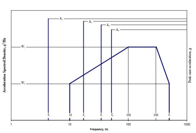
Figure 514.7C-9 from MIL-STD-810G w/ Change 1 – Helicopter Vibration Profile (Sine over Random)
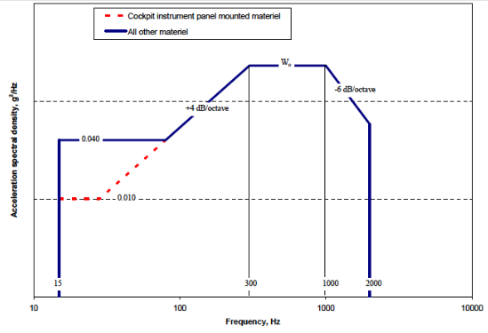
Figure 514.6C-6, Category 7 - Jet aircraft vibration exposure
Before we introduce the method of multi-resolution spectrum, all the vibration controllers in the market use FFT, a method which only provides linear frequency scale with uniformed resolution. In other words, what we do with the controller is not done the current industry.
Introducing Multi-Resolution Spectrum Analysis
The method of multi-resolution spectrum developed by Crystal Instruments is a modification to the single pass FFT. The basic concept is that it applies two or more passes of FFT to the same incoming time streams and create a synthesized spectrum in the frequency domain, where the frequency resolution varies. The following diagram shows how it works with two-pass FFT.
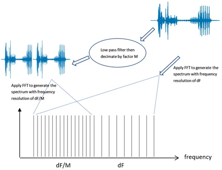
When multiple channels of time data continuously come in, the signal processor will take them by blocks simultaneously and transform the time blocks into frequency domain using FFT. At the same time, a decimation filter is applied to the original time stream and continuously generates the time stream at lower sampling rate. A second pass of FFT is applied to the time signals with lower sampling rate and creates the FFT spectrum at a finer resolution. Finally, the signal processor will combine the two banks of spectrum into one. The synthesized spectrum will have two different frequency resolution: one at dF and one at dF/M where M is the decimation factor.
The description above uses the most succinct language to describe this process. The actual implementation is very complex. There are many detail factors to consider, including:
How to deal with the overlapping processing?
What type of decimation filter to use, FIR or IIR?
What is the effect of filter delay of decimation filter?
What is the effect of phase distortion of decimation filter?
What decimation factor to choose from: 2, 4, 8 or any other number?
How should the average be applied to multiple passes of FFT?
What types of signals are adequate to this process and what types are not?
How will the data window be applied to multiple passes of time domain signals?
All of these details have been addressed in the Crystal Instruments products when multi-resolution spectrum method is applied. The software also takes care of the appropriate processing, storage, display and reporting for multi-resolution spectrum analysis.
The decimation process applies and generates continuous time streams. For this reason, multi-resolution spectrum analysis is more adequate for continuous signals than of transient signals. For example, the hammer test uses transient events to compute the FRFs, and thus would not be a good fit for multi-resolution spectrum analysis.
Applying the Multi-Resolution Spectrum Analysis in Structure Vibration Analysis
Modal Analysis
A modal test is carried out to compare the effect of multi-resolution and single resolution spectrum. The structure under test is a steel plate that is hung vertically using a bungee cord to produce a free-free boundary condition. The high-quality factor (Q) of the plate helps in observing the advantages of the multi-resolution spectrum. A white noise excitation from a modal shaker is used to excite the steel plate. The response of the plate is captured using a uni-axial accelerometer.
The test configuration details are described here. A sampling rate of 51.2 kHz is used for the interested analysis frequency range of 23 kHz. The block size of 4096 yields 1800 spectral lines which yields a frequency resolution of 12.5 Hz. A Hann window is used to reduce the leakage from the white noise excitation and response. A linear averaging mode of 32 is used to compute the linear spectrum.
An 8 times finer resolution of 1.56 Hz is obtained in the low-frequency range using the multi-resolution spectrum. This is achieved by using a large block size which is not needed in the high frequency region because of the dynamics of the test structure. This implementation of different resolutions produces better results without any increase in the loop time. The cutoff frequency dividing the low and high-frequency range is 2.8125 kHz. In this low-frequency region, the results from the multi-resolution tests are better because of the finer frequency resolution. After this cut-off frequency, the multi-resolution and single-resolution spectrum would yield comparable results since they have the same frequency resolution. All other settings, configurations and setup are the same for both multi-resolution and single-resolution tests.
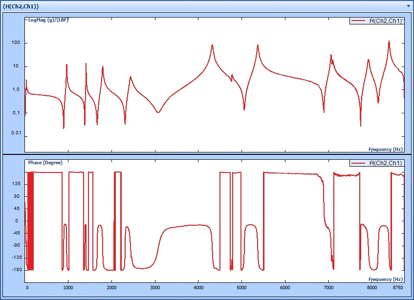
Following graph illustrates both the Multi resolution and Single resolution spectrum covering the whole frequency range.

Zooming into the high-resolution region of the Multi-resolution spectrum, and comparing to the single resolution, following spectrum graph is produced.
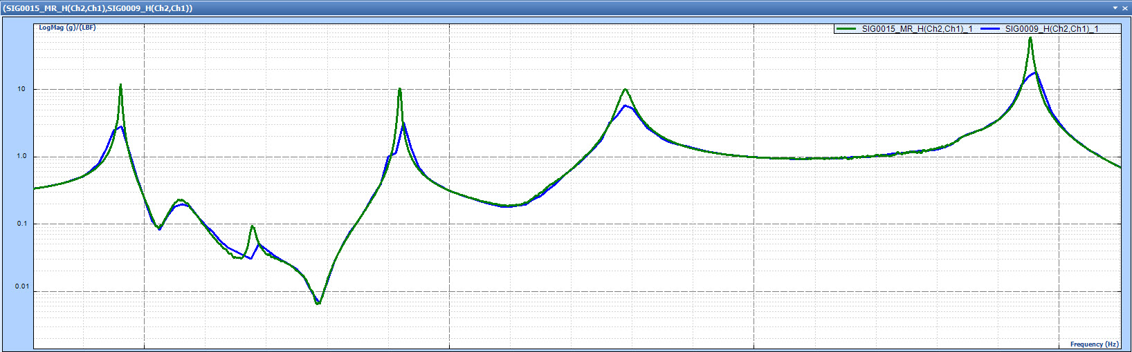
The image shows that in the cut-off frequency region, where the frequency resolution is much finer with the multi-resolution spectrum (green), the peaks at several resonance frequencies are much clearly identified. This is due to the much higher block size, which ultimately produces higher spectral lines. Therefore, the Frequency Response Function curve is much smoother and neater.
This also facilitates a more accurate calculation of the quality factor and peak amplitude of the FRF as shown in the table below. The table shows that the first four resonance frequencies that are present within the low-frequency cut-off region have a much higher Q and peak amplitude with the implemented multi-resolution spectrum. Also, in the high-frequency region, the frequency resolution for the single and multi-resolution spectrums are the same and hence the Q and peak amplitude for these resonances are also very close.
|
Resonant Frequency |
Q estimation using MR |
Q estimation using regular FFT |
FRF Amplitude Estimation using MR (g/LBF) |
FRF Amplitude Estimation using regular FFT (g/LBF) |
|
960.94 Hz |
311.069 |
40.138 |
12.269 |
2.832 |
|
1418.75 Hz |
313.292 |
120.452 |
10.687 |
3.274 |
|
1789.06 Hz |
97.435 |
52.326 |
9.993 |
5.823 |
|
2453.13 Hz |
461.059 |
89.479 |
60.277 |
18.42 |
|
5350 Hz |
126.317 |
126.19 |
33.72 |
34.74 |
|
8462.5 Hz |
172.296 |
185.73 |
32.08 |
31.47 |
|
12725 Hz |
94.498 |
88.965 |
186.23 |
187.72 |
The table above shows that the amplitude and Q factor estimation using regular FFT methods are off from their true values by an order of magnitude of tens or hundreds. If people use these erroneous values to derive their conclusion about the structure and conduct further analysis, such as structure modification and optimization, the results will of course be wrong.
Random Vibration Control
The method of multi-resolution spectrum analysis can be further extended into the control process. This means that the output signal computation will come from the measurement spectrum based on multi-resolution spectra.
To increase the control performance in the low-frequency range while maintaining a reasonable loop time, different resolutions can be applied to the low and high-frequency range in the entire control process.
In the implementation of Crystal Instruments Random controller, multi-resolution spectrum analysis is applied to all power spectrum calculation. It is then extended to computing the transfer function matrix and generating the drive signal that excites the shaker. Because the drive computation at low frequency band now contains more detail information, it will be able to control the structures at much higher resolution.
The user defined profile shall be decomposed into 2 bands in the initializing period, to get the low band reference profile. The Spider controller from Crystal Instruments will operate on these two profiles simultaneously.

In the composite windows below, a comparison is made between a test with and without multi-resolution spectrum control. The FFT line is set to 400. The frequency range is 2kHz. In the plot, the green line is the target profile. The black line is the conventional control spectrum signal at frequency resolution of 5Hz. The blue line is the one with multi-resolution turned on. The blue line has two resolutions in the whole frequency range: in high frequency band it is 5Hz, while in low frequency band it is 0.625Hz.
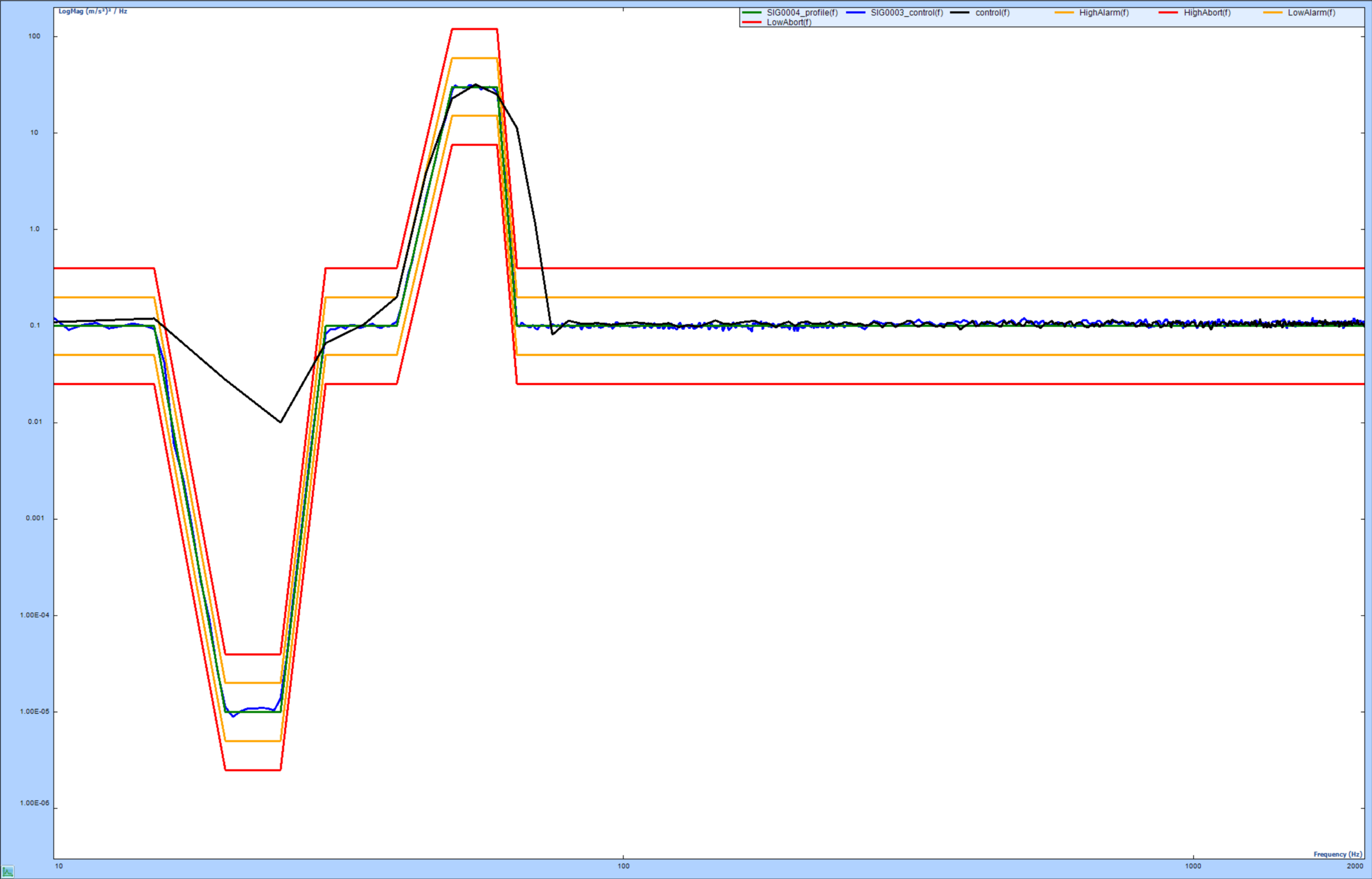
Or we can display the testing results separately.
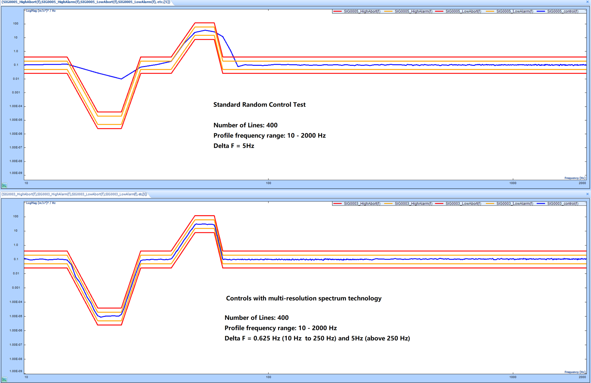
Obviously, the one with multi-resolution can achieve much better control dynamic range that that of without. It is common to see a 20dB or more improvement of the control dynamic range in the low frequency range.
Conclusion
The conventional signal processing algorithms used by the FFT signal analyzer may not match the requirements needed in the physical world. FFT, while having the benefits of efficient computation, only provides the spectrum with a uniform frequency resolution across the whole frequency range after the transform. On the other hand, many applications in the mechanical vibration and acoustics ask for finer frequency resolution at the lower frequency end.
The method of multi-resolution spectrum developed by Crystal Instruments can successfully generate a spectrum with two or more stages of frequency resolution. It has been successfully used in Random vibration control, general dynamic signal analysis and modal testing, offering a 100x improvement to the estimation accuracy.
References
[1]. Cooley, James W.; Tukey, John W. (1965). "An algorithm for the machine calculation of complex Fourier series". Mathematics of Computation. 19 (90): 297–301. doi:10.1090/S0025-5718-1965-0178586-1. ISSN 0025-5718.
[2]. Dynamic Signal Analysis Basics (Product Note #001, 32 pages, 1.1 MB, Crystal Instruments)
Describes the basic dynamic signal analysis theory including Fourier Transform, data windowing, linear spectrum, power spectrum, cross spectrum, FRF and coherence, averaging, transient capture and hammer test, overlapping process, SDOF system. Read online here.
[3]. V. Adams and A. Askenazi, Building Better Products with Finite Element Analysis, OnWord Press, Santa Fe, N.M., 1999.