Every multi-shaker random controller eventually has to answer one question: what drive signals will make the control points do what the test profile asks? Answering it means inverting the system's frequency response function (FRF) matrix at every spectral line. This inversion plays a role in maintaining stable MIMO control.

In MIMO random control in compliance with MIL-STD-810H Method 527.2, the Singular Value Decomposition (SVD) is the tool that makes this inversion safe. This article explains why direct matrix inversion can be risky, how SVD helps evaluate the shaker system, and how truncating small singular values improves control stability.

The control problem in one equation

A MIMO vibration system with n drives (shakers) and k control points (accelerometers) is described, line by line in frequency, by

𝐘𝜔=𝐇𝜔 𝐗𝜔

where X is the drive vector, Y is the control response vector and H is the k × n FRF matrix measured in the pretest. The controller knows the target linear spectrum T and needs the drive that produces it:

𝐓(𝜔)= 𝐇(𝜔) 𝐗(𝜔) ⇒ 𝐗(𝜔)= 𝐇⁻¹(𝜔) 𝐓(𝜔)

Ideally, this would be enough to calculate the drive signals. Typically, H is hard to invert because of the characteristics of the shaker system:

It may not be square. With more controls than drives (n < k) or more drives than controls (n > k), there is no ordinary inverse at all.

Even when n = k, as in the six-shaker test described below, H can be nearly singular at some frequencies.

Why a direct inverse is risky

A poorly conditioned FRF matrix can cause small measurement errors to become much bigger when calculating drive signals. In a shaker system, this can result in drive spikes, unstable control, or amplified noise. This can happen when:

several shakers excite similar structural modes, so their columns of H look alike;

a control point is only weakly coupled to the drives;

the structure has anti-resonances in the band;

measurement noise is present.

These conditions are common in multi-shaker vibration testing. On a 6DOF table, these conditions can happen at certain frequencies during 6DOF vibration testing, so the controller needs a way to identify and manage these conditions to maintain stability.

What SVD tells you about your shaker system

SVD splits the FRF matrix at each frequency into three pieces:

𝐇(𝜔)= 𝐔(𝜔) 𝚺(𝜔) 𝐕ᴴ(𝜔)

V holds the drive singular vectors: independent patterns of shaker drive.

U holds the response singular vectors: the control-point patterns those drive patterns produce.

Σ is diagonal, holding the singular values σ₁ ≥ σ₂ ≥ … ≥ σₙ (for n ≤ k).

Each singular value is the gain from one drive pattern to its response pattern. A large σ means the shakers move that pattern easily. A small σ means that pattern is hard to excite, so reaching it would take a large drive. This means that the singular values measure the controllability of each independent mode of the system. This works for both square and non-square H matrices, which is why one SVD-based least-squares solution covers the over-determined, exactly determined and under-determined cases.

Reading the condition number

The ratio of the largest to the smallest singular value is the condition number, which is a useful indicator of how sensitive H is to measurement errors:

κ(H) = σ_max σ_min

Condition number κ	What it means
< 10	Well conditioned
10–100	Acceptable
100–1000	Marginal; truncation typically begins here
> 1000	Unstable or poorly controllable

Plotted across the band, κ points straight at the frequencies where control will struggle, usually near anti-resonances or where multiple shakers excite similar structural modes.

Truncation: drop the modes you can't control

The pseudo-inverse built from the SVD inverts each singular value:

𝐇⁺(𝜔)= 𝐕(𝜔) 𝚺⁺(𝜔) 𝐔ᴴ(𝜔)

This can create a problem because when σ is very small, 1/σ becomes very large, which can lead to excessive drive signals. So the controller uses a truncated version, Σₜ⁺, which removes singular values below a threshold:

H⁺(ω) = V(ω) Σ_t⁺(ω) U^H(ω), σ_i < ασ_max ⇒ removed, α ≈ 0.01 ∼ 0.05

In effect, the controller stops trying to drive the modes it cannot control well. The main benefits:

reduced drive amplification;

improved control stability;

lower sensitivity to noise.

However, there is a trade-off: perfect tracking of the control specification may no longer be possible for the truncated modes. This helps limit drive amplitudes and maintain control stability.

SVD inside the closed loop

The truncated pseudo-inverse is not used once and forgotten. It runs at every step of the control loop.

Initial drive. From the target linear spectrum: X(ω) = H⁺(ω) T(ω).
Error. The controller compares the measured control PSD with the target PSD, converts that PSD error into a linear-spectrum magnitude error, and combines it with the measured phase into a complex error vector e(ω) = T(ω) − Y(ω).
Correction. The same truncated pseudo-inverse maps the error back to the drives: ΔX(ω) = H⁺(ω) e(ω).
Update. Xₖ₊₁(ω) = Xₖ(ω) + ΔX(ω), and the loop repeats until the end of the test.

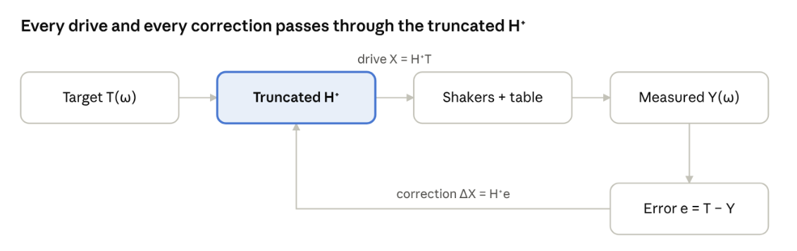
closed-loop MIMO control · drive and correction both use H⁺

Because the correction also goes through H⁺, errors related to poorly controllable modes can be prevented from producing extremely large drive corrections.

The controller can also re-estimate H from running data, H_new = G_yx G_xx⁻¹, to track nonlinearities and structural changes. Often times, both are used together: FRF updates for model accuracy, drive iteration for fast convergence. One caution: with highly correlated control profiles the measured response space can become effectively rank-deficient. FRF updates from closed-loop data then become less reliable, and disabling FRF adaptation can give more robust control.

Results from a Six-Shaker 6DOF Test

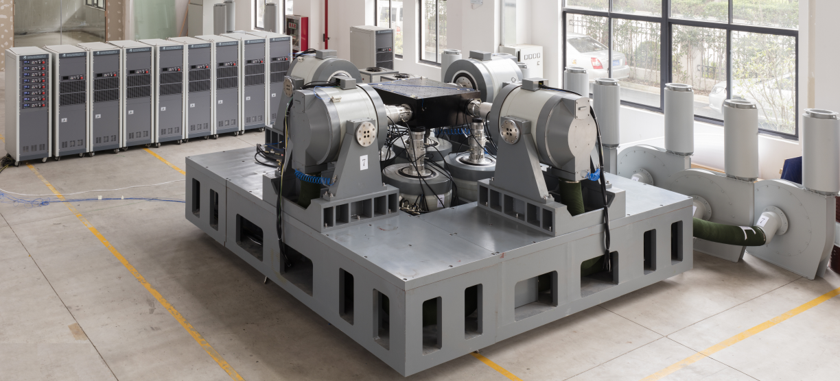
We ran a 10–500 Hz, 800-line MIMO random test on a six-shaker MET sub-configuration of an eight-shaker 6DOF table: one X, two Y and three Z shakers, with six control accelerometers in the same 1X / 2Y / 3Z arrangement. With singular-value truncation suppressing poorly conditioned modes, all six control PSDs converged within about 1 dB of their targets across the band.

The takeaways for anyone running multi-shaker control:

Look at the singular values, not just the FRFs. They tell you which motions your shaker layout can actually produce.

Watch the condition number. It flags the frequencies where control will be hard before you run the test.

Truncate deliberately. Even though tracking accuracy can be reduced for poorly controllable modes, this helps keep drive signals within limits and maintain control stability.

Want to learn more? Email us at info@go-ci.com for more information.

Why SVD Keeps MIMO Vibration Control Stable